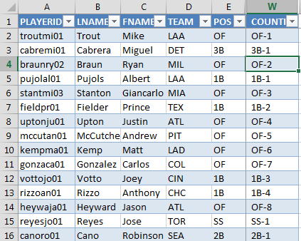
I just came across an interesting use of an Excel formula that will let you easily determine what a player’s ranking is at their given position (1B-1, 1B-2, 1B-3, etc.).
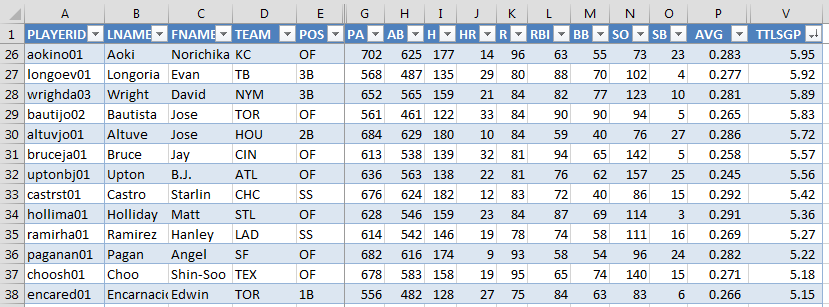
Here’s an explanation that might show what I’m talking about. You’re scrolling through your huge list of ranked hitters (see image below). You have them sorted by Total Standings Gain Points (column V) in descending order.
You see Edwin Encarnacion’s name pop up in row #38. You know he’s a first basemen, and you can pretty easily determine that he must be the #37th ranked player (by showing up on row 38). But now you want to know where he ranks amongst only other first basemen.

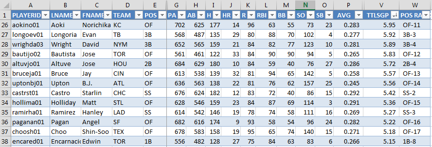
In this post I’ll show you a formula we can use to get our spreadsheet to look like this (look at column W):
I’m a Moron
I got nearly to the end of this post when I started to think it was weird that Encarnacion was ranked #37, Starlin Castro #32, and Paul Goldschmidt #21. Turns out I used a rankings file from the 2013 preseason for all the screenshots…
I decided against starting over because it’s not the player names that are important, we’re mostly looking at a new formula. And I found it pretty interesting and thought provoking to look at these old lists and see names like Nori Aoki and B.J. Upton so high.
Excel Formulas Used In This Post
Using the “&” to Build Text
As you can see from the image above, we’re trying to take each player’s position (e.g. “1B”) and then add a dash and then the player’s positional ranking (e.g. “1B-8” for Encarnacion).
You can use the ampersand (would you know what that was called without “Wheel of Fortune”?), in an Excel formula to add text from different columns.
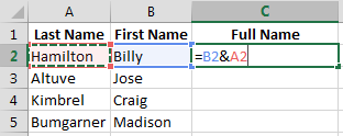
A real practical application of this is to build a player’s full name (e.g Billy Hamilton) from their first name and last names being in separate columns. Here’s an example:
 Continue reading “How To Add Positional Ranking To Your Spreadsheet”
