Welcome to the third part of the “How To Calculate Rankings For a Points League” series in which we’ll go step-by-step through the process of using Microsoft Excel to calculate your own rankings for a fantasy baseball points league (as opposed to rotisserie or head-to-head rotisserie).
If you’re looking for info on how to rank players for a roto league, look here.
I recommend going through all the parts of the series in order. If you missed an earlier part of this series, you can find it here:
ABOUT THESE INSTRUCTIONS
- The projections used in this series are the Steamer 2015 preseason projections from Fangraphs. If you see projections that you disagree with or that appear unusual, it’s likely because I began writing this series in December 2014, still early in the off-season.
- For optimal results, you will want to be on Excel 2007 or higher. Some of the features used were not in existence in older versions.
- I use Excel 2013 for the screenshots included in the instructions. There may be some subtle differences between Excel 2007, 2010, and 2013.
- I can’t guarantee that all of formulas used in this series will work in Excel for Mac computers. I apologize for this. I don’t understand why Excel operates differently and has different features on different platforms.
IN PART 3
In this part of the series we’ll use Excel’s VLOOKUP and IFERROR formulas as well as Table and Structured Reference features to pull hitter information and projections from other areas of the spreadsheet in order to create our hitter rankings tab.
EXCEL FUNCTIONS AND FORMULAS IN THIS POST
Below are the Excel functions and formulas used in this part of the series. If you’re already familiar with what these are, you can skip ahead to the step-by-step instructions.
VLOOKUP
One of the most powerful Excel formulas, in my opinion. And it’s easier to use than you might think.
This formula searches the first column of a table for a desired value (a player ID) and then returns a value that is in the same row but in a separate column. For example, we might tell Excel to go into a table of projection data, locate the player ID for Billy Hamilton (10199), and give us back the number in the fourteenth column (column N, which holds the number of SBs).

This formula requires four inputs:
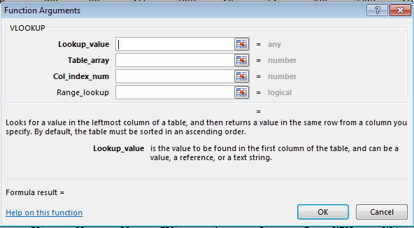
VLOOKUP(lookup_value, table_array, col_index_num, range_lookup)
- Lookup_value – This is the value we want to search for in the table of data (e.g. Billy Hamilton’s player ID 10199). In the rankings spreadsheet, we’re mostly going to use player IDs for this. “Hey Excel, go look for this player ID”.
- Table_array – This has to be two or more columns of data. Excel will look for the Look_up value in the first column in the set of data. You do not necessarily need to include the first column on a spreadsheet tab (you don’t have to use Column A of a sheet, the first column of your table could be Column G). But Excel is going to look through the first column you provide. “Hey Excel, here are fifteen columns of data for you, look through everything in the first column for the Lookup_value.”
- Col_index_num – This is the column number that of the Table_array that contains your desired information. This has to be a number and it has to be within the Table_array you provided. For example, if your table_array only has five columns, but you put a six for Col_index_num, you’ll have a problem. “Hey Excel, the fourteenth column has projected stolen bases. After you find Billy Hamilton’s player ID, tell me how many stolen bases are in that fourteenth column.”
- Range_lookup – This input can be either “TRUE” or “FALSE”. If you use “TRUE”, Excel will look for an approximate match of the lookup_value (PLAYERID). If you enter “FALSE”, Excel will only look for an exact match. This is an optional input, but I feel very strongly that it must be used and that “FALSE” is the option selected. You may otherwise get the wrong projections showing up for players.
TABLES (NAMED RANGES, Structured References)
Similar to how we named individual cells in the last part of our series, Excel has functionality that allows you to convert a block of data (player projections) into a named table. There are quite a few benefits to using tables:
- Tables have names. This is great for the Table_array input in the VLOOKUP formula. We can give the projection sheet the name “STEAMER_H” (for Steamer Hitters projections) and use that instead of traditional way of selecting data in Excel (something like’Steamer Hitters’!A1:W500). Not only is this a huge time saver (using your mouse to scroll and select 20 columns and 500 rows takes a long time), but it gives your formulas meaning. When you look back at your VLOOKUP formula and see “STEAMER_H”, you’ll easily be able to remember that you’re looking up projected Steamer hitter information.
- Columns have names. I have a hard time remembering what column projected HRs are in. But I don’t need to if I know that the column name is “HR”. If you don’t use a table, you’re stuck trying to remember things like, “were HRs in column G, H, or I?”. And then you have to figure out if column I is column number 8, 9, or 10? When referring to a column, use the following convention – TABLENAME[COLUMNNAME]. The column name is surrounded in brackets.
- Formula consistency. In a table, all formulas within a column are identical. When you change the formula in one cell of a column, the rest of the column automatically updates too. No more editing a formula in one cell and having to copy it to hundreds of other cells in the same column.
- Easy sorting and filtering. As easy as clicking a drop down arrow.

COlumn
This function returns the column number of a cell or range of data. The function only requires one input; the cell or range to be evaluated:
COLUMN(TableName[ColumnName])
Let’s use a real example to illustrate:
COLUMN(STEAMER_H[SB])
This formula will look for the stolen bases column in the Steamer Hitter Projections and will return the column number. If SB are in column N, this formula calculates to 14.
IFERROR
The IFFERROR function allows us to control what happens when another formula being used is calculating out to an error.
The image below is a great example of this. In this spreadsheet we have a series of VLOOKUP formulas that instruct Excel to go find Kendrys Morales’ player ID (moralke01) in the “Steamer Projections” tab.
You may recall that during the 2014 season Morales remained an unsigned free agent until well into the season, so he was not included in the Steamer projections. Because he was not included, the VLOOKUP formula could not find his player ID and could only calculate to this “#N/A” error message.

The IFERROR function will allow us to replace the error message with any value of our choice. It essentially works by telling Excel, “If this other formula I’m using comes back with an error, use this instead”.
Using IFERROR we could instead make Kendrys Morales line look like this:

The formula requires two inputs:
IFERROR(value,value_if_error)
- Value – This represents the formula or calculation we want Excel to perform. In our example above it will be the same VLOOKUP formula we already have entered.
- Value_if_error – This represents the value or message we want Excel to return if the first argument, “Value”, happens to be an error. In our example above we don’t want the default “#N/A” error message that turns up if Excel cannot locate Kendrys Morales in the RoS projections. Instead, we could just ask for Excel to return zeroes for his projected stats.
STEP-BY-STEP INSTRUCTIONS
(more…)
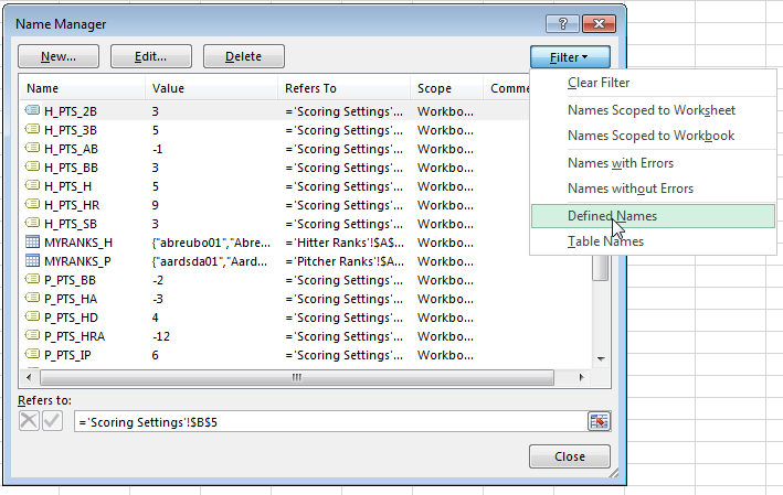
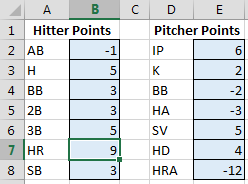 To refresh your memory and to see the complete list of named cells, access the “Formulas” tab of the Ribbon and then click the “Name Manager” button.
