How To Calculate Custom Rankings for a Points League: Part 3 – VLOOKUP, Excel Tables, and Structured References

Welcome to the third part of the “How To Calculate Rankings For a Points League” series in which we’ll go step-by-step through the process of using Microsoft Excel to calculate your own rankings for a fantasy baseball points league (as opposed to rotisserie or head-to-head rotisserie).

If you’re looking for info on how to rank players for a roto league, look here.

I recommend going through all the parts of the series in order. If you missed an earlier part of this series, you can find it here:

ABOUT THESE INSTRUCTIONS

  • The projections used in this series are the Steamer 2015 preseason projections from Fangraphs.  If you see projections that you disagree with or that appear unusual, it’s likely because I began writing this series in December 2014, still early in the off-season.
  • For optimal results, you will want to be on Excel 2007 or higher.  Some of the features used were not in existence in older versions.
  • I use Excel 2013 for the screenshots included in the instructions.  There may be some subtle differences between Excel 2007, 2010, and 2013.
  • I can’t guarantee that all of formulas used in this series will work in Excel for Mac computers.  I apologize for this.  I don’t understand why Excel operates differently and has different features on different platforms.

IN PART 3

In this part of the series we’ll use Excel’s VLOOKUP and IFERROR formulas as well as Table and Structured Reference features to pull hitter information and projections from other areas of the spreadsheet in order to create our hitter rankings tab.

EXCEL FUNCTIONS AND FORMULAS IN THIS POST

Below are the Excel functions and formulas used in this part of the series. If you’re already familiar with what these are, you can skip ahead to the step-by-step instructions.

VLOOKUP

One of the most powerful Excel formulas, in my opinion. And it’s easier to use than you might think.

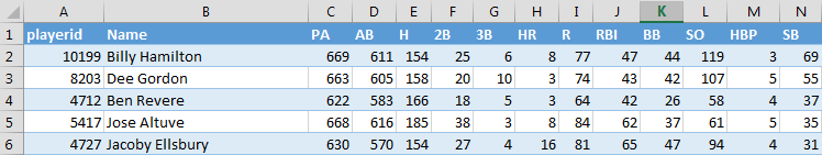
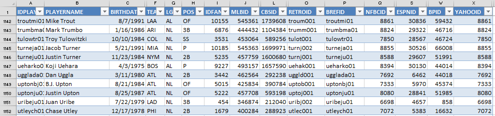
This formula searches the first column of a table for a desired value (a player ID) and then returns a value that is in the same row but in a separate column. For example, we might tell Excel to go into a table of projection data, locate the player ID for Billy Hamilton (10199), and give us back the number in the fourteenth column (column N, which holds the number of SBs).

BILLY_HAMILTON_PROJ_SB

This formula requires four inputs:

VLOOKUP(lookup_value, table_array, col_index_num, range_lookup)VLOOKUP

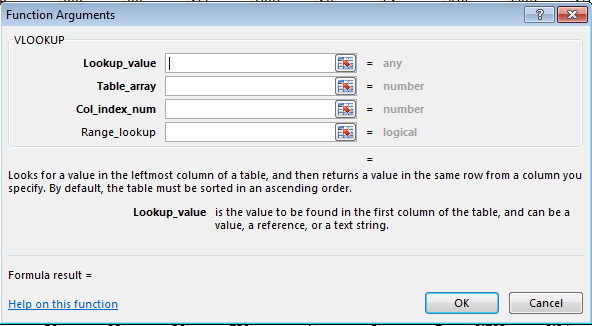
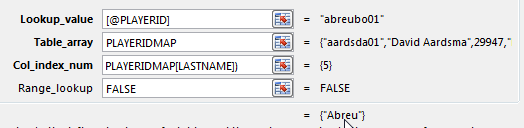
  1. Lookup_value – This is the value we want to search for in the table of data (e.g. Billy Hamilton’s player ID 10199). In the rankings spreadsheet, we’re mostly going to use player IDs for this. “Hey Excel, go look for this player ID”.
  2. Table_array – This has to be two or more columns of data. Excel will look for the Look_up value in the first column in the set of data. You do not necessarily need to include the first column on a spreadsheet tab (you don’t have to use Column A of a sheet, the first column of your table could be Column G). But Excel is going to look through the first column you provide. “Hey Excel, here are fifteen columns of data for you, look through everything in the first column for the Lookup_value.”
  3. Col_index_num – This is the column number that of the Table_array that contains your desired information. This has to be a number and it has to be within the Table_array you provided. For example, if your table_array only has five columns, but you put a six for Col_index_num, you’ll have a problem. “Hey Excel, the fourteenth column has projected stolen bases. After you find Billy Hamilton’s player ID, tell me how many stolen bases are in that fourteenth column.”
  4. Range_lookup – This input can be either “TRUE” or “FALSE”. If you use “TRUE”, Excel will look for an approximate match of the lookup_value (PLAYERID). If you enter “FALSE”, Excel will only look for an exact match. This is an optional input, but I feel very strongly that it must be used and that “FALSE” is the option selected. You may otherwise get the wrong projections showing up for players.

TABLES (NAMED RANGES, Structured References)

Similar to how we named individual cells in the last part of our series, Excel has functionality that allows you to convert a block of data (player projections) into a named table. There are quite a few benefits to using tables:

  1. Tables have names.  This is great for the Table_array input in the VLOOKUP formula. We can give the projection sheet the name “STEAMER_H” (for Steamer Hitters projections) and use that instead of traditional way of selecting data in Excel (something like’Steamer Hitters’!A1:W500).  Not only is this a huge time saver (using your mouse to scroll and select 20 columns and 500 rows takes a long time), but it gives your formulas meaning.  When you look back at your VLOOKUP formula and see “STEAMER_H”, you’ll easily be able to remember that you’re looking up projected Steamer hitter information.
  2. Columns have names. I have a hard time remembering what column projected HRs are in. But I don’t need to if I know that the column name is “HR”. If you don’t use a table, you’re stuck trying to remember things like, “were HRs in column G, H, or I?”. And then you have to figure out if column I is column number 8, 9, or 10?  When referring to a column, use the following convention – TABLENAME[COLUMNNAME]. The column name is surrounded in brackets.
  3. Formula consistency. In a table, all formulas within a column are identical. When you change the formula in one cell of a column, the rest of the column automatically updates too. No more editing a formula in one cell and having to copy it to hundreds of other cells in the same column.
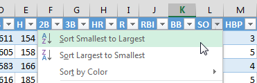
  4. Easy sorting and filtering. As easy as clicking a drop down arrow.EXCEL_TABLE_SORT

COlumn

This function returns the column number of a cell or range of data. The function only requires one input; the cell or range to be evaluated:

COLUMN(TableName[ColumnName])

Let’s use a real example to illustrate:

COLUMN(STEAMER_H[SB])

This formula will look for the stolen bases column in the Steamer Hitter Projections and will return the column number.  If SB are in column N, this formula calculates to 14.

IFERROR

The IFFERROR function allows us to control what happens when another formula being used is calculating out to an error.

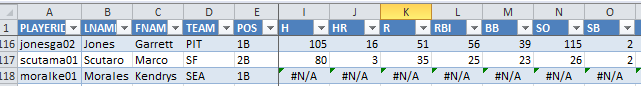
The image below is a great example of this. In this spreadsheet we have a series of VLOOKUP formulas that instruct Excel to go find Kendrys Morales’ player ID (moralke01) in the “Steamer Projections” tab.

You may recall that during the 2014 season Morales remained an unsigned free agent until well into the season, so he was not included in the Steamer projections. Because he was not included, the VLOOKUP formula could not find his player ID and could only calculate to this “#N/A” error message.

IFERROR-Excel-Formula

The IFERROR function will allow us to replace the error message with any value of our choice. It essentially works by telling Excel, “If this other formula I’m using comes back with an error, use this instead”.

Using IFERROR we could instead make Kendrys Morales line look like this:

KENDRYS_MORALES_IFERROR

The formula requires two inputs:

IFERROR(value,value_if_error)

  1. Value – This represents the formula or calculation we want Excel to perform. In our example above it will be the same VLOOKUP formula we already have entered.
  2. Value_if_error – This represents the value or message we want Excel to return if the first argument, “Value”, happens to be an error. In our example above we don’t want the default “#N/A” error message that turns up if Excel cannot locate Kendrys Morales in the RoS projections. Instead, we could just ask for Excel to return zeroes for his projected stats.

STEP-BY-STEP INSTRUCTIONS

Continue reading “How To Calculate Custom Rankings for a Points League: Part 3 – VLOOKUP, Excel Tables, and Structured References”

How To Calculate Custom Rankings for a Points League: Part 2 – Set Up League Scoring Settings

Welcome to the second part of a series in which we’ll go step-by-step through the process of using Microsoft Excel to calculate your own rankings for a fantasy baseball points league (as opposed to rotisserie or head-to-head rotisserie).

Whether you’re in a standard points league at a major site like ESPN or a more advanced Ottoneu league at Fangraphs, this process will help you develop customized rankings for your league.  These instructions can be used for a season-long points league or a weekly head-to-head points league.

If you’re looking for info on how to rank players for a roto league, look here.

I recommend going through all the parts of the series in order. If you missed Part 1 of this series, where we downloaded hitter and pitcher projections and started to set up the rankings Excel file, you can find it here.

About These Instructions

  • The projections used in this series are the Steamer 2015 preseason projections from Fangraphs.  If you see projections that you disagree with or that appear unusual, it’s likely because I began writing this series in December 2014, still early in the off-season.
  • For optimal results, you will want to be on Excel 2007 or higher.  Some of the features used were not in existence in older versions.
  • I use Excel 2013 for the screenshots included in the instructions.  There may be some subtle differences between Excel 2007, 2010, and 2013.
  • I can’t guarantee that all of formulas used in this series will work in Excel for Mac computers.  I apologize for this.  I don’t understand why Excel operates differently and has different features on different platforms.

In Part 2

In this second part of the series, we’ll create a new tab in our Excel file to document our league’s scoring settings.  We’ll use Excel’s “Name” feature so we can calculate projected points for all players and easily make changes to the scoring system in the future.

Excel Functions and Formulas In This Post

Below are the Excel functions and formulas used in this part of the series.  If you’re already familiar with what these are, you can skip ahead.

Named Cells (or Named Ranges)

Excel has a feature called “Names”, where you can give a cell, a group of cells, or an entire table a name.  After giving a cell a name, you can then use the name in calculations.

In this part of the series we’ll give names to the point values of each scoring category for our league. Let’s assume each HR for a hitter is worth 9 points.All_Point_Values

We can name this point value as “H_PTS_HR”.

If we’re later trying to determine how many points Javier Baez will earn from home runs, we can multiply Baez’s projected home runs by “H_PTS_HR” instead of multiplying by 9 or by cell B7 (in the image above).
Javier_Baez_HR

If you’re familiar with the basic concepts of computer programming, setting the point value of home runs equal to a name is like using a variable.

The benefit of this is that we can later change the 9 to a different value. This is especially useful if we play in multiple leagues or if the scoring format changes.

It becomes very easy to change the scoring system without having to search within complex formulas. And we also don’t need to flip back and forth and remember that the HR point value was in B7 (as opposed to B6 or B8).

Using a name also gives the formula “meaning”.  It’s a lot easier to understand this:

= B2 * H_PTS_HR

than it is to understand this:

= B2 * B7

Another helpful benefit is that Excel makes all of your Names available through a type-ahead feature.  So if you know you have a series of Names that start with “H_PTS_”, you can see all of them by typing out part of the name. This works no matter what tab of the Excel file you are on, meaning you don’t have to flip back and forth to figure out the exact cell holding the point value.

List_Of_Names_H

Using Cell Shading To Indicate Meaning

As we continue to build a spreadsheet that will eventually be quite complex, it can be helpful to indicate which cells are “input” cells and which ones are “calculated” (formula) cells. An easy way to denote this is by using cell shading (or coloring).

An “input” cell would be facts or assumptions that will later be used in formulas for calculating projected points and player rankings.  For example, the number of points for each home run hit or the number of teams in the league.

A “calculated” cell will obviously be some kind of formula we enter in Excel.

The color coding will help remind you what cells you can change in the future (inputs) and what cells you should leave alone (formulas, calculations).

You can use your own color scheme, but for the rest of the series I will shade cells blue if they are “input” cells and a light red if they are “calculated” cells.

Not to mention that color coding your spreadsheets also offers a nice intimidation factor to your opponents at the draft table.  Who knows, someone might just think twice about getting in a bidding war with you if you’ve got a kick ass spreadsheet on-screen.

Adjust For Your League’s Scoring Settings

The example league I’m using to create these rankings for is loosely based on a scoring system suggested for Fangraphs Ottoneu leagues.  It is likely very different than the scoring system in your league.  Accordingly, you will need to use judgment and tailor the steps below to fit your league’s specific scoring system.

STEP-BY-STEP INSTRUCTIONS

Continue reading “How To Calculate Custom Rankings for a Points League: Part 2 – Set Up League Scoring Settings”

How To Calculate Custom Rankings for a Points League: Part 1 – Download Projection Data and Player ID Map

Welcome to the first part of a series in which we’ll go step-by-step through the process of using Microsoft Excel to calculate your own rankings for a fantasy baseball points league (as opposed to rotisserie or head-to-head rotisserie).

Whether you’re in a standard points league at a major site like ESPN or a more advanced Ottoneu league at Fangraphs, this process will help you develop customized rankings for your league.  These instructions can be used for a season-long points league or a weekly head-to-head points league.

If you’re looking for info on how to rank players for a roto league, look here.

In this first part of the series we’ll start a new Excel file and download projection information.

Why I Created This Series

Points leagues seem to be like fingerprints and snow flakes. Each one is a little different than the others. I’m a big believer that in order to be a strong fantasy player, you need to create your own rankings and dollar value calculations that are tailored specifically to the league(s) you play in.

I’ve also felt that nobody takes the time to explain exactly how to create your own rankings. If you look hard enough you might find an article that gives a quick bullet point list.  Maybe something like:

  • Download projections
  • Multiply projections by your point system
  • Adjust for replacement level
  • You’re done!

I’m going to be a little more thorough than that.

In Part 1

In this first part of the series we’ll download hitter and pitcher projections, take a look at and download player ID information, and bring all of this information into one Excel file.

ABOUT THESE INSTRUCTIONS

  • The projections used in this series are the Steamer 2015 preseason projections from Fangraphs.  If you see projections that you disagree with or that appear unusual, it’s likely because I began writing this series in December 2014, still early in the off-season.
  • For optimal results, you will want to be on Excel 2007 or higher.  Some of the features used were not in existence in older versions.
  • I use Excel 2013 for the screenshots included in the instructions.  There may be some subtle differences between Excel 2007, 2010, and 2013.
  • I can’t guarantee that all of formulas used in this series will work in Excel for Mac computers.  I apologize for this.  I don’t understand why Excel operates differently and has different features on different platforms.

Where To Get Projections

There are many solid projection systems available for download.  Some very fine projections are available at membership sites like Baseball Prospectus or Baseball HQ.

But if you’re like me, when I started out on the adventure of calculating my own rankings, I wasn’t looking to pay for something I wasn’t sure I’d be able to translate into fantasy success.  It’s great to have accurate projections, but how do you use them if you can’t take the next step to rank and value those projections?

For that reason, I’m partial to the Steamer projections.

They’re available in easy-to-use Excel downloads (specifically CSV) at Fangraphs. There are also daily rest-of-season updates, meaning on any day you can see the projections for the remainder of the season for any player.  Steamer does a good job of projecting playing time (if a player gets hurt, they try to estimate the effect on playing time).

And they’re free.

Use Whatever Projection System You Prefer

I’ll be using Steamer in this example.  But you can use the system of your choice.  Just try to pick a system that uses some form of player ID system.

What is a Player ID?

Just like you and I are identified by Social Security Numbers or employee IDs (at work), most of your major fantasy or MLB websites use some form of an ID number that is unique to each player.

Using an ID is a more reliable way of identifying a player than a simple name.  Two players can have the exact same name (think Chris Young and Alex Gonzalez) which could cause big problems when ranking players.

And players can go by different name variations (Mike and Michael, Jon and Jonathan, JP and J.P., AJ and A.J.) or even change their name (Mike to Giancarlo Stanton, Fausto Carmona to Roberto Hernandez).

Here’s a quick look at some player IDs for various systems:

Player ID Source Mike Trout Clayton Kershaw Giancarlo Stanton
Baseball Reference troutmi01 kershcl01 stantmi03
Fangraphs 10155 2036 4949
MLB 545361 477132 519317
CBS 1739608 1221725 1630093
ESPN 30836 28963 30583

If you’re wondering how to determine someone’s player ID, visit their player page on a particular website.  You can usually find the player ID in that web page’s URL.  For example, here’s Mike Trout’s MLB.com player page:

MIKE_TROUT_PLAYERID

In looking at that table above, you can see here that there is not one universal numbering system.

To alleviate this problem, I maintain a “Player ID Map” (click here to download in Excel).  The Player ID Map lists out all “fantasy-relevant” players and their ID for each of the major systems (Fangraphs, Baseball Reference, Baseball Prospectus, Yahoo, ESPN, etc.).

PlayerIDImage

I stumbled across the concept of the player map from Tim Blaker at Crunchtimebaseball.com and tailored it to meet my needs.  This provided me with an excellent starting point.  Tim maintains his own version and updates his more frequently than I do.  I only maintain my own because I’ve wanted to add some new columns.

On this site I will typically work with the Baseball Reference ID.  I like those IDs more than the others because I can look at an ID and usually determine who the player is (troutmi01 is Mike Trout).  Most other sites use a straight ID number that has no inherent meaning (10155 or 545361).

If you’re familiar with Excel and using VLOOKUPs, Player IDs are the item we’ll be matching upon to start pulling information around our Excel rankings file.  If you have no idea what I just said, don’t worry.  We’ll get there soon.

STEP-BY-STEP INSTRUCTIONS

Continue reading “How To Calculate Custom Rankings for a Points League: Part 1 – Download Projection Data and Player ID Map”

Are Hitter SGPs Directly Comparable to Pitcher SGPs?

I recently got an e-mail from a reader of the site (thanks Brad!), asking an interesting question. He was working through creating his own standings gain points rankings and tailoring them for his custom league.

How do I bring Losses into the SGP calculation? If I do make losses a negative, how would I make the pitcher and hitter SGP numbers apples-to-apples?

You might realize that he actually has the correct answer, but it didn’t make sense at first because he wanted to keep hitter and pitcher SGP comparable.

Losses Are an Inverse Category

Losses, like ERA and WHIP, is a category where the goal is to have the lowest total. So the answer is to make the SGP factor a negative number.  If you think about how we calculate SGP factors, we’re really trying to find the slope, or line of best fit, to our historical standings data.

Stolen_Bases_SGP
Example SGP slope calculation.

Traditional categories like Ws and Ks have a line with a positive slope (slanting up and to the right on your high school math class x- and y-axis).  The higher the number of Ws on the x-axis, the more points you get in the standings on the y-axis.

The slope of a graph plotting out Losses would be downward sloping.  The more Ls on the x-axis, the lower the standings points reflected on the y-axis.

So Brad had the right answer, but he was afraid that adding in another inverse pitching category was going to destroy his ability to compare hitter and pitcher SGPs.

The Real Reason We’re Here

I realize you didn’t come here for me to take you back to basic math class.  The real question is, can you take a pitcher who is projected for 4 SGP and say he’s a better draft selection than a hitter projected for 3.8 SGP? Continue reading “Are Hitter SGPs Directly Comparable to Pitcher SGPs?”

How To Calculate Projected Standings For Your Draft

So you’ve got a great set of projections, rankings, and dollar values.

This is great for draft preparation. But how do you take this information and use it during the draft?  Is there a way to monitor the progress of the draft and see if you’re lacking in power compared to the others in the league?  Do you need speed?  Are you lacking in strikeouts?

You don’t need to buy draft software or a special draft spreadsheet.  You can easily add a few more things to your Excel files and have a very powerful draft tool that can help you make these assessments.

I wrote about how to track drafted players in a spreadsheet last January.  If you haven’t read that yet, please do.  The instructions that follow pick up where that post leaves off.

Here’s how to calculate projected standings during your draft.

Prerequisites

I’ll be using Excel 2013 to create the projected standings.  I think you’ll be able to follow a very similar process in Excel 2010 and Excel 2007.

Teams_Drafted
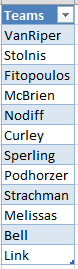
As I mentioned, this post assumes you have already added the named range and data validation drop down listing to select the team that has drafted a player.

This is how you will be tracking the draft selections during your draft.  As each player is taken, you’ll locate them on your rankings/projections lists and select the team that drafted them.

I realize it’s a little early to be thinking about draft spreadsheets, but it’s top of mind for me now because I am participating in a mock draft that was coordinated by Bryan Curley of BaseballProf.com.  I wanted to see how the draft is going and how teams stack up after the first few rounds.  Not to mention you can set this up in your spreadsheet now and have it read to roll when we finally get closer to the season.

You can see the list of those participating in the mock draft in image above.  As selections are being made in the draft, I’m marking them off in drop down I created in the “TAKEN” column.TAKEN


You may want to make several “fake” selections in your Excel file, just to have some data to work with.  You will want to test that your projected standings are working prior to the draft…  That’s the last thing you need to be monkeying on draft night.

Excel Functions and Features We’ll Be Using

There are a variety of ways to do this, but I’ll show you how to use a pivot table in this example.  If you’ve never created a pivot table before, don’t worry.  They’re a lot easier to work with than most think.

The pivot table will help us to quickly accumulate every team’s offensive stats (R, RBI, HR, SB, BA).  Once we have the statistics accumulated in one nice table, we’ll then use the RANK formula to calculate the standings.

Pivot Tables

Pivot tables are very useful for taking a lot of lines of data (like we have on our “Hitter Ranks” tab) and combining or summarizing that data into more easily or digestible parts.

For example, your listing of all hitters and their projections is probably hundreds of rows of information.  If you were to select 14 hitters for each of the 12-teams in your league, that would be 168 hitters.  Sorting all of those players into teams and then calculating the totals for five different categories for each team might seem like a daunting task.

The good news is that creating a pivot table can be done in only a few clicks of the mouse and within minutes you can have a table that looks just like this:

Pivot_Table_Projected_Standings

Rank (or RANK.EQ) Formula

These two formulas are essentially the same; however, RANK was discontinued in Excel 2010 and was replaced by RANK.EQ.

If you’re using Excel 2010 or later, either one should work. But if you are using Excel 2007 or earlier, you must use RANK (RANK.EQ didn’t exist then).

These formulas will interpret a list of numbers and return the ranking of a specified item in the list.  We can use this to analyze the entire list of player SGPs and give us a ranking for each player (e.g. Mike Trout is #1).

The formulas require three inputs:

RANK(Number, Ref, Order)

RANK.EQ(Number, Ref, Order)

  1. Number – This is the specific number you want ranked. If your goal is to figure out where your team ranks in total home runs, you would select the individual cell containing your team’s projected home runs.
  2. Ref – This is the range of data, or the list of data, to calculate the ranking from. Continuing with the total home runs example, you would select the entire listing (or range) of projected home runs for all teams in the league.
  3. Order – Technically this is not a required part of the formula, but using it can make our lives a little easier. If you leave this part out of the formula, Excel would return a “1” for the team with the most home runs and a “12” for the team with the least home runs. You can see we don’t really want to know our “Rank”. We’re looking for “Rotisserie Points”. We would like the top team in home runs to show a “12”. The “Order” parameter in the RANK function is looking for a zero or a one. If you leave it blank or put in a zero, the RANK function gives a “descending” ranking. This is the typical ranking where “#1” is the best or highest possible ranking. We are looking for an “ascending” ranking, where a “12” is the best result. To do this, just put a one in for this piece of the function.

Step-by-Step Instructions

Continue reading “How To Calculate Projected Standings For Your Draft”

How to Use Excel to Determine Replacement Level

Who is the replacement level shortstop in a 12-team league that starts one shortstop and one middle infield position?

We know there will be at least 12 shortstops drafted in this scenario.  But will there be 15, 16, 17, 18, or more drafted?  And where does that put the replacement level shortstop at?

This concept of replacement level has always been a little bit of a problem for me.  In my original series about ranking players, I mentioned that in this 12-team scenario, that we would have 36 combined 2B and SS drafted, and to simplify things we could assume that would be 18 second basemen and 18 shorststops.

But that’s not a precise enough answer.

If we’re trying to squeeze every drop of value from our drafts, we should determine precisely who the replacement level player is at each position.  After all, replacement level is a huge driver in the calculation of a player’s value.

So we need to get it right.

What You Can Expect

I’m going to show you a system I’ve started using that will help you identify:

  • The starters at each position (e.g. top 12 1B, top 60 OF, etc.)
  • The corner and middle infielders (the next 12 best 1B/3B and 2B/SS)
  • The 12 utility players (the next 12 best players at any position)
  • The replacement level player at each position

The system is very easy to do.  I was forced to come up with it out of necessity when I was working on my recent analysis of the past five years of draft results.  For that post I had to calculate projected and actual dollar values for each of the last five seasons. So I needed a fool-proof method for determining replacement level 10 times in a short period of time and I also wanted to be able to come back to each set of data and easily be able to tell what group each player fell into.  Thus the color coding.

Replacement_Level
Here’s a little taste of what we’re going to do. I’ll show you a process that will take you only a few minutes to color code and clearly document players into groups of Starters, CI/MI, UTIL, and Replacement Level.

Excel Features You Should Know

There are three pretty neat features of Excel that I used during this process that you may not be familiar with, and they might be able to save you a lot of time: Continue reading “How to Use Excel to Determine Replacement Level”

Now in Amazon – Using Standings Gain Points To Rank and Value Players


The Kindle edition of “Using Standings Gain Points to Rank and Value Fantasy Baseball Players: A Step-by-Step Guide Using Microsoft Excel” is now available at Amazon.com.

Want an edge in your league?  Click here to get started on creating customized rankings and dollar values tailored specifically to your league.

The book contains 150+ pages of detailed instructions, over 200 screenshots of how to build this powerful Excel spreadsheet, and links to download 10 example files.

Is There a Hitting / Pitching Split for a Points League?

I recently started working on my next book looking at how to create customized rankings and dollar values for a points league.  For the most part, much of the same principles followed for ranking players in a rotisserie league still apply.  But then I stumbled upon a major difference, one that I can’t find guidance on anywhere.

Points Leagues Cut Right To The Chase

One really nice thing about points leagues is that the goal is much more straightforward than in a roto league.  Instead of trying to compose a balanced team in the 10 different categories of a rotisserie league, you’re really just competing in one category… total points.

Because of this, we can cut through some of the exercises we have to do for ranking a roto league.  We don’t have to mess around with league history, determine Standings Gain Points for each category, and don’t have to convert each player’s projections into SGP.

We Just Have To Calculate Projected Points For Each Player, Right?

This is the biggest task, for sure.  Make sure to build in a replacement level calculation, too.

I think that’s what most people would do and just stop there.  But if you want an edge, I think we can dig a little deeper.

Quickly, Here’s How I Would Calculate Projected Points

I’m going to go into much more detail in the finished guide and include screenshots, tips, and tricks to make this a spreadsheet you can use into the future.  But here’s the high level:

  1. Download a set of reliable projections
  2. Document your league’s scoring settings (e.g. 10 points for a HR, 2 for SB, etc.)
  3. Multiply the projected stats by your scoring settings
  4. Determine and adjust for replacement level

Follow these steps and you’ll end up with the total number of “useful” or “draftable” points.

Why Do We Have a Rotisserie Split?

Continue reading “Is There a Hitting / Pitching Split for a Points League?”

How Do You Account For and Value Players with Multiple Position Eligibility?

Zobrist_Prado_Santana_Carpenter
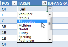
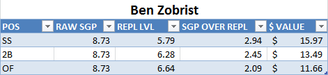
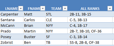
How do we handle the multi-position players like Ben Zobrist and Martin Prado?  When a player is eligible to be slotted at 2B, SS, and OF, how do we value that player?

This question came up in the comments of my last post on “How to Add Positional Ranking to Your Spreadsheet“, from a reader named Michael (I welcome your questions too).  In this post I’ll take a look at how I handle this and look at a more inticate approach you could take to get the information.

I must warn you that it takes a lot of new formulas and manipulation of your existing rankings spreadsheet to accommodate multiple positions.  To make sure you have something to reference, at the end of this post I’ll provide a download link to an example Excel file you can download.

Assign the Player to the Weakest Position They’re Eligible For

This is what I currently do.  For example, let’s take a player like Ben Zobrist, who in the 2014 season currently qualifies at SS, 2B, and OF.

In the Player ID Map, I attempt to classify each player at the weakest position they’re eligible for.  I do that by determining what replacement level is for a standard 12-team mixed rotisserie league.

Is the “weakest position” going to be the same for every league?  No it’s not.  It’s probably close in most leagues.  Catcher will almost surely be the weakest in any format.  Then Shortstop will generally be the next weakest, followed by 2B, 3B, 1B, and OF.  But positions might change a little in an 8-team league or a 15-team league, in an AL-only league versus a standard league.

That’s a big reason why I started this site.  It’s not always safe to give blanket advice, and I think the best approach is to calculate all of these things for your own league.  You’ll be better off for it.

How Do I Determine the Weakest Positions?

Assuming you’ve done some kind of work to create your own rankings (if not, start here), the weakest position can easily be determined by looking at the replacement level information you’ve calculated (if you want to refresh your memory on replacement level, read this).

Looking back to one of my preseason files for the 2014 season, this is the replacement level information for one of my leagues.
REPL_LEVEL_TABLE

The weaker positions are those with the lowest replacement level.  So in this league it’s C, SS, 2B, and then 1B, 3B, and OF are essentially the same.

Back to Zobrist

Going back to our example of Ben Zobrist who is eligible at SS, 2B, and OF, if we’re trying to assign him to the weakest position he’s eligible for, he would be assigned to SS.

Thinking of Martin Prado who is eligible at 2B, 3B, and OF, he would be assigned to 2B.

Carlos Santana who is eligible at 3B and C would be assigned to C.

Why Do I Only Assign a Player to One Position?

I have two reasons for this.

The main reason is because assigning players to the weakest position they are eligible for gives the player his greatest value.  I’ll demonstrate more on this in a minute.  But if you’re calculating Zobrist’s dollar value, it comes out highest when he’s classified as a SS.

Going along with this, fantasy baseball leagues are becoming more efficient market places.  As we all get better and smarter about playing fake baseball, people generally realize they’re best off putting Buster Posey at catcher and not at 1B.

This won’t always be the case, but for the most part the obvious situations like your Buster Poseys and Carlos Santanas are going to be assigned where they belong.  Because of this, it’s somewhat of a wasted effort to try calculating values for them at 1B or 3B.

The second reason is a technological one.  You run into a lot of trouble having the same player appear multiple times in one spreadsheet (on multiple rows).  Not only does it become confusing to have to remember that Zobrist’s name appears three times in your draft list, but it also greatly complicates (or eliminates) your ability to calculate dollar values.

How Much Does a Player’s Position Affect Their Value?

Is there really a big difference between a SS and an OF?  Let’s take a look.

I am running the exercise below using Steamer’s 2014 preseason projections.  The dollar values assume a 12-team standard mixed rotisserie league with 14 hitters (C, C, 1B, 2B, 3B, SS, CI, MI, OF, OF, OF, OF, OF, UTIL) and 9 pitchers.  The dollar values are calculated using standings gain points and my approach to calculating player values.

Here’s the replacement level information again:REPL_LEVEL_TABLE

Let’s start out with Zobrist.  You can see below that he was projected for 8.73 SGP before adjusting for replacement level.  When you then account for replacement level and figure out his “SGP Over Replacement Level” you see that he becomes much more valuable as a shortstop.  Over $4 more valuable than when he’s classified as an OF!

BEN_ZOBRIST_REPL_LEVEL Continue reading “How Do You Account For and Value Players with Multiple Position Eligibility?”

An Even Better Positional Ranking Formula

In my last post about how to calculate positional rankings in your player spreadsheet (link), I realized a weakness in the approach I outlined.  I’m here to fix that with a slightly more complex formula. Final_Excel_Formula_Output

The Weakness In The First Approach

The problem with the first approach is that it is entirely dependent upon how the file is sorted.  If the file is sorted by dollar value or standings gain points in descending order, then the rankings work.

But if you sort the file by home runs, stolen bases, or player name, then the rankings fall apart.  The player with the most home runs (or the most stolen bases or the first name alphabetically) becomes the top ranked player.

The COUNTIFS Excel Function

Instead of the COUNTIF function, we’ll use the COUNTIFS function this time.

You might remember from the last post that the COUNTIF function will count the number of cells in a specific range that meet a specified condition (e.g. “Hey Excel, count all the players in this column that have a ‘POS’ of ‘OF’.”).

Well the COUNTIFS function counts the number of cells in a specific range that meet all of the conditions you provide (you can give multiple conditions).

In plain English, our goal is to have Excel count all the players in our list of hitters that have a “POS” of “OF” AND that have a higher projected SGP than our player being evaluated.

We’ll get into the specifics of our formula in a bit, but here’s a screenshot of the Excel formula wizard for our COUNTIFS function.COUNTIFS_FUNCTION

This formula allows for an open-ended number of arguments, but you do need to pieces of information for each set of criteria you want to specify.  Each criteria requires:

  1. Range – This is the block, column, or area of cells we want to count from.  “Excel, look in Column E and count the cells that meet this condition I’m about to tell you about in bullet #2.”
  2. Criteria – This is what we are evaluating the cells for.  “Count the cells in Column E that show ’1B’ as the position.”

If we want to specify three conditions that must be met, then we would need six arguments (three ranges and three criteria: range1, criteria1, range2, criteria2, range3, criteria3).

Step By Step Instructions

Continue reading “An Even Better Positional Ranking Formula”