I think you’re gonna like this one.
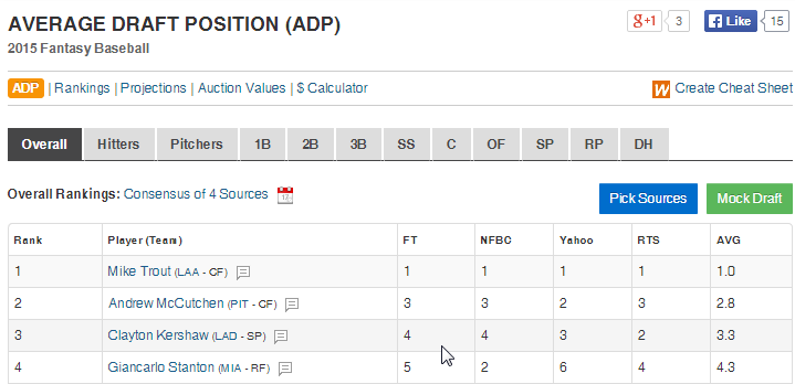
In this post I’ll show you how to link live average draft position information from the web into your draft spreadsheet. Every time you open your rankings file it will pull down updated ADP information. Bam!
How We’re Going To Do This
We will use a powerful feature of Excel called web querying to pull in the ADP information aggregated by FantasyPros.com (please note, I’m an affiliate of Fantasy Pros). The web query will suck up that table of ADP information and bring it directly into Excel for us to then VLOOKUP into our existing “Hitter Ranks” and “Pitcher Ranks” tabs.
Assumptions
I am assuming that you’ve followed my Standings Gain Points or Points-League Ranking series and are already starting with a spreadsheet that is based off one of those (you don’t have to have those exact spreadsheets, but something similar).
Excel Functions and Concepts Used in this Post
Web Query
As you can probably imagine, the power of the web query is that it automatically updates the data in your Excel file without you having to do ANYTHING after the initial setup.
Web queries are created from the “Data” tab on the Excel Ribbon, under the “Get External Data” icon grouping. There are several ways to get data from outside sources into Excel, we will be using the “From Web” button.

One “weakness” I have found in web queries is that they cannot work with “tables” in Excel. You cannot pull a web query in as the data of a table. If you’re a big follower of this site you know that’s a bit of an issue for me because I use tables all the time. Thankfully this doesn’t prevent us from doing things, I just point it out because you might wonder why I set things up the way I do in the instructions below.
Find
The FIND function searches within a specified cell for a string of text that you provide. If the FIND function locates the string, it will return the character position where the string starts at.
I know, you’re thinking “What the heck does that even mean?”. Here’s an example. Let’s say we have the text “Mike Trout (LAA)” in a cell and every player in our whole spreadsheet follows that format. If we want to pull out each player’s team we will need to start by figuring out where the team name starts in that cell. And we can’t just say it will always start at the 13th character each time when we have players like this hanging around MLB.
Instead we can use the FIND formula to intelligently determine where that opening parenthesis is for each player (it starts at 12 for Trout and 23 for Salty).
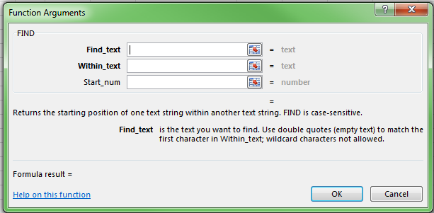
This formula requires two inputs:
FIND(Find_text, Within_text)
-
Find_text – This is the string of text you are searching for and keep in mind it is case-sensitive. You would wrap the string you are searching for in quotation marks. So in our example above, to look for the opening parenthesis you would enter “(” here. Or if you’re trying to be slightly more precise, you could enter ” (“, a space before the parenthesis.
-
Within_text – This is the text you want to search WITHIN. This can be a cell number.
Left
The LEFT function gives you the leftmost number of characters in a text string. You also get to specify the number of characters to specify.
For example, if you have a text string of “Mike Trout (LAA)” and you ask for the 10 leftmost characters in that string, you would get “Mike Trout” back.
This formula requires two inputs:
LEFT(Text, Num_chars)
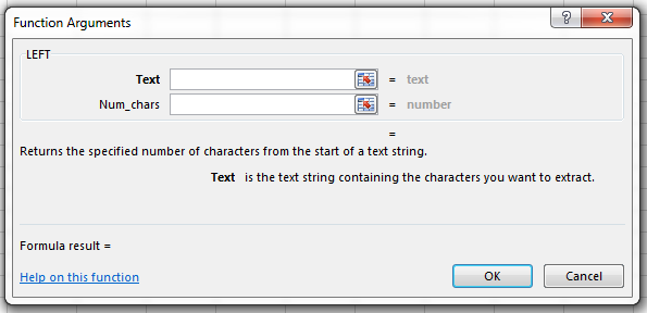
- Text – This is the text string you want the leftmost characters from.
-
Num_chars – This is the number of characters you want from the string. This can be a hard entered number (e.g. 10) or it can be a formula itself that results in a number.
Combining Functions Together
We can do something pretty powerful by combining the FIND and LEFT functions together. I’ve been hinting at it with this “Mike Trout (LAA)” example. Recall from above that the LEFT function wants to know our text string (“Mike Trout (LAA)”) and the number of characters on the left to pull from that string.
Assume that cell B2 has a value of “Mike Trout (LAA)”. Instead of using this formula:
LEFT(B2, 10)
We can use this:
LEFT(B2, FIND(" (",B2)-1)
The FIND(" (",B2)-1 part of the formula returns a 10 (if you don’t subtract the one it returns an 11), and “Mike Trout” has 10 characters in it (including the space). By using this combination of functions we don’t have to type in a “10” for Mike Trout and a “21” for Saltalamacchia.
Important Prerequisite
Before you’re able to proceed with the instructions below you must make sure the PLAYERIDMAP in the file you’re working with was updated after February 21st, 2015. I added a column to the Player ID Map called “FANTPROSNAME” that is necessary for the steps below to work.
Instructions for updating your PLAYERIDMAP can be found here. Completing the update should only take five minutes or so.


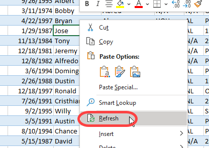

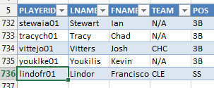

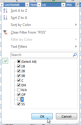
 Copy this information and go to your “Hitter Ranks” tab and paste it into the first cell below the header in column A there.
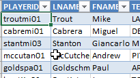



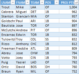
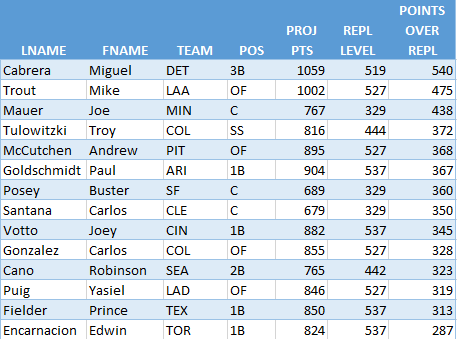

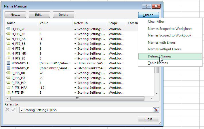
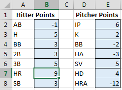 To refresh your memory and to see the complete list of named cells, access the “Formulas” tab of the Ribbon and then click the “Name Manager” button.
