How to Add Batter and Pitcher Handedness to your Daily Fantasy Baseball Spreadsheets

In this post I’ll show you how to add batter and pitcher handedness to your spreadsheets. To do this, we’ll have to learn two new Excel formulas we have not tackled yet.

I’ve avoided doing this for a long time… But there’s just no way around it now. It’s time to say goodbye to relying exclusively on VLOOKUP. Let’s put on our big boy pants and tackle VLOOKUP’s more flexible and powerful counterpart… INDEX and MATCH.

Sometimes VLOOKUP Can’t Get the Job Done

Take this scenario. You’ve started to build a DFS spreadsheet and you’ve imported FanDuel player salaries from a CSV file. Now you want to add player handedness (Lefty/Righty) as a column to your spreadsheet.

You are also aware of the Player ID Map and know that it’s an easy way to get handedness information on players.

You look at this data above and you think, “No problem!”. FanDuel ID is in both sets of data. How hard could this be? A simple VLOOKUP and we’re done.

But you quickly realize things are not that easy. You see, the VLOOKUP has a very restrictive assumption. If you are doing a VLOOKUP from the salary information into the Player ID Map, the Excel function assumes that “FanDuelID” will be the FIRST column in the Player ID Map.

And that’s NOT the case.

Let’s look at an example VLOOKUP formula:

In this formula we’ve told Excel to go look for the “FanDuelID” column in the “PLAYERIDMAP” table and give us back the value in the 10th column.

But “FanDuelID” is not the first column of the PLAYERIDMAP. It’s the 33rd (wow… the Player ID Map is getting to be quite large). So VLOOKUP will not work.

Other Weaknesses of VLOOKUP

Not only is assuming the data you want to match is in the first column awfully restrictive, if you think about it, VLOOKUP also ties you to a left-to-right lookup. For example, if you’re trying to use Excel to VLOOKUP which team Michael Brantley plays for, his player ID must be in the first column of your data set and you are then forced in to looking only to the right.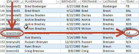

We want a formula that will allow our lookup to be in any column and then to look to the left! For example, go find Nelson Cruz’s FanDuelID and then look to the left a few columns and give me the side of the plate he bats from.

Going back to this example formula right above, the hard coding of a “10” in the formula to return the information in the 10th column is a flimsy approach, but that’s how many people are taught to write VLOOKUP formulas.

The flimsiness comes in if you decide to insert a column somewhere in the PLAYERIDMAP. If column 10 becomes column 11, Excel will not adjust its formula accordingly. Because you are likely building a spreadsheet that you’ll use all throughout the season, it seems highly likely you’ll want to add a new piece of information to your analysis. That inevitably means adding columns to bring that new information in. You don’t want to have to hunt through your formulas to figure out what the new column number in your VLOOKUP needs to be.

Enter “INDEX” and “MATCH”

That’s right. To defeat the almighty VLOOKUP formula, we need to combine the powers of two functions (that last sentence just made me think of this). Let’s take a look.

INDEX

When I’m using a function I’m unfamiliar with, I will add it through the “Insert Function” button. I like doing this because Excel will then give you a search menu to find a formula. And after locating your function you’ll get a helpful wizard that breaks down all the inputs it needs.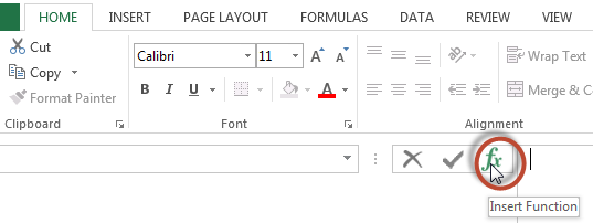

If you follow that approach to add the INDEX function, you’ll soon realize there are two versions of it.

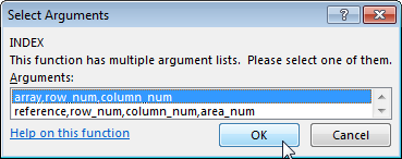
I always use the first version, which allows us to locate a cell anywhere within a block of data and return the value from that cell. This function uses the following inputs:

1. Array – The range of cells you are searching for a value in. This could be a table or a block of cells.
2. Row_num – The row within that array that the value is in. This should be a number representing the row.
3. Column_num – The column within the array that the value is in. Again, this should be a number representing the column (not the letter representation of the column).

It may help to see a visual representation of the function. Assume we’re trying to find Nelson Cruz’s batting handedness. If we tell the index function to look in the PLAYERIDMAP (the “array”), in row 309 (“row_num”), and column 26 (column_num), it would return “R”.

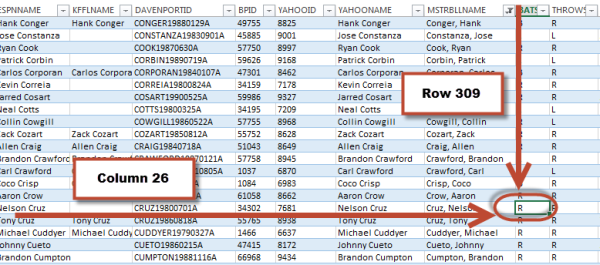
We know the array to look in. And we can easily determine the column we want to look in. The challenge we now face is how to determine the row to look in… How do we easily determine that Nelson Cruz is listed on row 309. That’s where the “MATCH” function can help us.

MATCH

The MATCH function will look for a specific value in a range of cells. The function will return a number representing where the matched item falls in the list.

Translating that into English, a realistic use for the function is to look in an entire column for a match. The function will start at the top of the column and proceed down until it locates the desired value. The function then returns where the item falls in the list, which happens to be the row the item is in.

The function uses these inputs:

1. Lookup_value – This is the value you are hoping to match in the array (or column). For us, this will usually be a Player ID of some sort.
2. Lookup_array – This is the area you are searching for the match within. When using the MATCH function with the INDEX function, this will usually be a column of data.
3. Match_type – This is an optional input telling Excel some more details about the kind of match you are looking for. You can enter a 1, 0, or -1. Entering a 1 or -1 are forms of approximate matches and are useful if you are looking up numeric values. But we are typically looking to match strings (I consider a Player ID made up of all numbers to still be a string) of text.

   This means we want exact matches only. Accordingly, I always use a 0 for this argument (even though it’s optional, leaving it blank tells Excel an approximate match is acceptable).

Combining INDEX and MATCH

As I alluded to before, the power of these two formulas comes when you combine (or nest) them together. Recall that the INDEX function looks like this:

If we drop the MATCH function in place of the “Row_num” argument:

We now have a formula that is more flexible and powerful than a VLOOKUP! The combination of INDEX and MATCH can look for a value anywhere in a table of data and we are no longer tied to the first column and a right-only lookup.

Step-by-Step Instructions

Lets go through the example scenario proposed above. We have a table of FanDuel salary information and we want to pull in handedness information from the Player ID Map.

Prerequisites

I am assuming you have already started an Excel file based off a FanDuel CSV export. If not, you can read how to do that here.

Step	Description
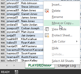
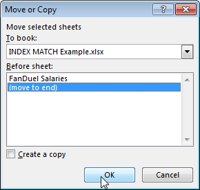
1.	Open your Excel file containing FanDuel salary information. Then download and open the SFBB Player ID Map (click that link and it should begin to download).  Once you’ve opened the Player ID Map, right-click on the “PLAYERIDMAP” tab and choose “Move or Copy…”. In the “Move or Copy” menu, select your FanDuel salaries spreadsheet in the “To book:” drop down menu (we’re copying the Player ID Map into the FanDuel salaries file). Choose the “[move to end]” option and click “OK”.
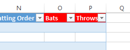
2.	Return to the tab containing the salary information and add two new columns. You can do this simply by typing your column name in the first row of the open columns. If your FanDuel CSV file is the same as mine, my first open columns are “O” and “P”. In cell “O1” type “Bats” and in cell “P1” type “Throws”. These are the columns we’ll use to pull in each player’s hitting and throwing handedness. As soon as you type in these cells Excel should automatically bring them in as part of the table and shade them (another benefit of using Excel tables). I shaded these columns red to indicate this information is coming from another source. This is just a small visual cue to let me know that columns A through N are from my FanDuel CSV and columns O and P are now coming from somewhere else. I have also sorted my spreadsheet by “Salary” in descending order so I can see names I recognize toward the top.
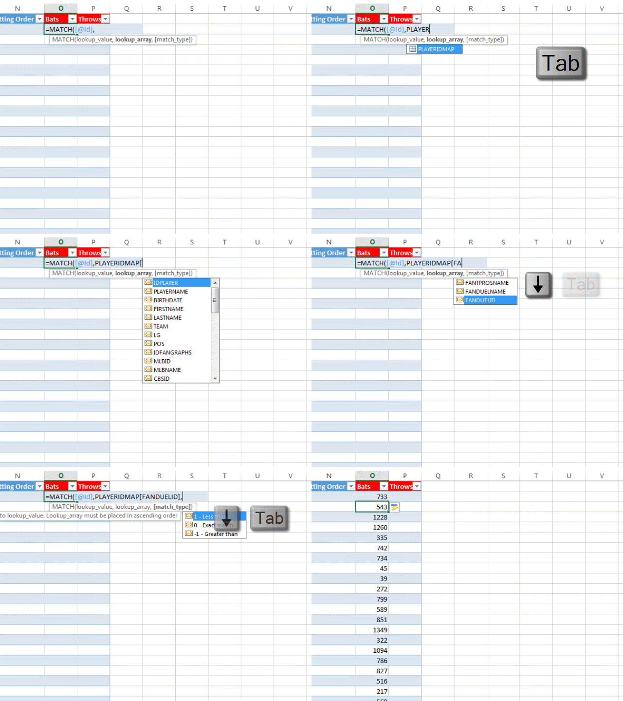
3.	Now it’s time to add our newly learned INDEX and MATCH formula. As I mentioned above, we need to embed the MATCH formula inside of the INDEX formula. We could attempt to write that one complicated formula right now, but I find it a lot easier to start small and expand my formulas rather than trying to write them all at once. And to do this I also find it easier to work from the inside out (another example of this is to start with a VLOOKUP formula first and then add IFERROR around it). So let’s start with MATCH. Start to type the following into the first empty cell in your “Bats” column: =MATCH( At this point you should see Excel recognize the formula and display the inputs needed to make it work. The first input is the lookup_value. Our goal is to look up a player’s FanDuel ID in our salaries list and locate the same ID in the “FANDUELID” column of the “PLAYERIDMAP” table. To reflect this, simply click on cell A2, which should contain the FanDuel ID of the first player listed (Clayton Kershaw in my file). Because we are using tables, Excel should automatically translate cell A2 to become “[@Id]”, which is the convention for referring to a value in the same row but in the “Id” column.
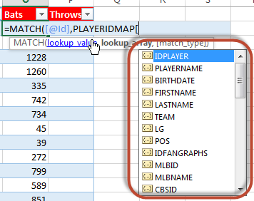
4.	Type a comma after the “[@Id]” input. The next input for the MATCH function is the lookup_array, which is where we want to find the FanDuel ID. In this scenario we are going to look within the “PLAYERIDMAP” and more specifically within the “FANDUELID” column. Start to type “PLAYERIDMAP” after your existing formula and you should see Excel recognize the table name we’re trying to refer to: When you notice that Excel has recognized what you’re going to type, hit the Tab key and Excel will complete the item for you. This is called “type ahead”. Let’s keep using this type ahead benefit to tell Excel we want the “FANDUELID” column of the “PLAYERIDMAP”. Type a “[” and you will be presented with a list of all the fields (or columns) in the “PLAYERIDMAP”. Use your up and down arrow keys to cycle through the list of fields. When you find the “FANDUELID” column, hit the Tab key to select it for the formula. After you have selected the column, type a the closing bracket (“]”) and a comma to end the lookup_array argument. Finally, type a “0” in for the match_type argument and close the entire MATCH formula with an ending parenthesis and hit ENTER. Your complete MATCH formula should be: =MATCH([@Id],PLAYERIDMAP[FANDUELID],0)
5.	After you complete the formula, you should see Excel automatically copy that formula to all the players below. Scroll through the list to make sure it appears to be working properly.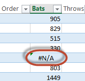 It’s very likely (inevitable) that you’ll find players displaying a “#N/A” error message. This doesn’t mean there’s an error in your formula. It means that the FanDuel ID was not located in the PLAYERIDMAP table. This is because I only aim to keep the list updated with “fantasy relevant” players. So bench players, non-impact rookies, and role players won’t be listed in the Player ID Map. Even if these players aren’t going to enter our DFS lineups, we still need to handle this error message, but let’s table it for now and come back to it later.
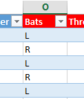
6.	Remember that the MATCH formula we just finished is an input into the INDEX function we will now use. Specifically, the MATCH function is the second input (Row_num) in the INDEX function: INDEX(Array, Row_num, Column_num) The first input, Array, is going to be “PLAYERIDMAP”. And the last input, Column_num, is the column number representing the batter handedness within the PLAYERIDMAP table. The “BATS” column, indicating batter hitting handedness, is in column AA of the Player ID Map, or the 27th column. To wrap the INDEX formula around the MATCH formula, type the edits in red below: =INDEX(PLAYERIDMAP,MATCH([@Id], PLAYERIDMAP[FANDUELID],0),27) After making that edit, you should now see batter information coming into the column. If you want to get really fancy, the hard coded “27” in the formula can be replaced with a formula that will determine that “Bats” is in the 27th column. Swapping out the “27” for this formula in blue will prevent problems down the line if the “Bats” column gets shifted into another column: =INDEX(PLAYERIDMAP,MATCH([@Id], PLAYERIDMAP[FANDUELID],0),COLUMN(PLAYERIDMAP[BATS])) Excel’s type ahead feature can still be used while editing things, even though other parts of the function have been tailored properly. I’ve written previously on the COLUMN function. You can read more about it and see another example of its use here.
7.	Now let’s revisit the players that are displaying errors in this column. Leaving errors here could lead to more errors further down the line if we base future formulas on this handedness column. The IFERROR function is ideal for handling lookup errors like these. It’s also very easy to use. Simply wrap the IFERROR formula around your existing formula, and give one more input outlining the text or message you want to display if there is an error in the formula. You can read more about IFERROR here. Let’s say we just want to leave the “BAT” column blank if an error is encountered. Entering two double quote marks consecutively will tell Excel to give a blank cell. With this our formula becomes: =IFERROR(INDEX(PLAYERIDMAP,MATCH([@Id], PLAYERIDMAP[FANDUELID],0),COLUMN(PLAYERIDMAP[BATS])),"") I realize the formula is getting to be a little out of control at this point. If you’re having a hard time understanding what is going on, try using the tip on complicated formulas shown below this table of instructions. Any formula that previously was resulting in an error will now show as a blank item.
8.	To create the formula for throwing (or pitching) hand, start by copying one of the cells in the “Bats” column. Note, do not “drag” the formula using the black box in the lower right hand corner of the selected cell. If you drag a formula that’s in an Excel table, the formula will adjust for the fact that you’ve moved it this way. Just like when you copy any normal Excel formula, the relative row and column references will change. There is no way to enter absolute cell references in table formulas that I’m aware of (these are the “$” symbols you might put in an Excel formula so cell references don’t shift as the formula is moved). But if you copy and paste a formula, the cell references don’t change!
9.	Because we haven’t changed the formula, the results in the “Bats” and “Throws” columns will be identical. So now just make the simple edit or replacing “BATS” with “THROWS” and you’ll be done! =IFERROR(INDEX(PLAYERIDMAP,MATCH([@Id], PLAYERIDMAP[FANDUELID],0),COLUMN(PLAYERIDMAP[THROWS])),"")

When It Makes Sense To Use INDEX & MATCH

If you’re a long time reader of the site, up until now (whether it’s creating SGP rankings, in-season rankings, or points league rankings) we haven’t merged more than one set of data together.

I’ve only relied upon Baseball-Reference IDs (like kershcl01 for Clayton Kershaw) to lookup Fangraphs’ Player IDs and because of that, VLOOKUP always worked. That’s because the Baseball-Reference IDs are in the first column of the Player ID Map. A necessity for VLOOKUP.

But now that we are letting other Player ID systems run the show (FanDuel IDs) and we need to look in columns that are to the left of our main ID system, we need INDEX and MATCH to make things work.

Tip If You’re Struggling

If you find that you’re having a difficult time layering all of these formulas on top of each other, try using multiple columns in Excel to build your formulas. You can have a column for each of the main formula components:

1. BatsMatch – Holds the Match formula
2. BatsIndex – Holds the Index formula and uses BatsMatch as one of the inputs
3. Bats – Is really just the IFERROR formula

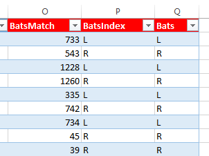
Here’s what each of the formulas would be:

BatsMatch: =MATCH([@Id],PLAYERIDMAP[FANDUELID],0)

BatsIndex: =INDEX(PLAYERIDMAP,[@BatsMatch],COLUMN(PLAYERIDMAP[BATS]))

BatsIndex: =IFERROR([@BatsIndex],"")

Instead of having lengthy formulas, these just reference and build upon one another.

What’s Next?

It’s going to be a bit of a challenge. But I think the next domino to fall has to be getting the opposing pitcher to show up in our file somewhere. We need starting pitcher to be able to determine which splits to use from our hitters and also to determine the quality of the overall matchup.

The FanDuel CSV file actually gives probably starting pitchers. We could just use formulas to pluck out the starter in each contest. But there’s no such information in Draft Kings’ exports.

I’m sure some of you are ahead of me in developing you spreadsheets. What websites are you pulling matchup information for? Keep in mind that we most likely want to find starting pitcher matchups for TOMORROW’s games. Not just the current slate of games. My goal is to provide an opportunity to start building a lineup a day in advance.

Thank you for following the site! Stay smart.