How to Use Excel Text Manipulation Formulas with Fantasy Baseball Data

In our last post we took a close look at a handful of different web query options available in Microsoft Excel.

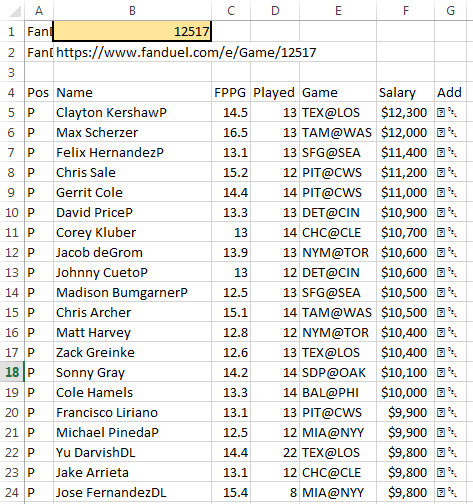
By the end of that post we had an Excel file that was able to automatically go out and pull in a raw listing of player names and salaries. All you had to do was figure out the ID for the slate of games you’re entering on FanDuel and type in that five digit number.

Then voila… Current salary information (or you can even run it for tomorrow to start planning the night before)!

The Next Step

So now we have player names and salaries. And we know from doing research at how to succeed playing DFS that we also need to bring in other information like batting and pitching splits, Vegas over/unders, and weather data.

We also know that using Player IDs is a more reliable way of matching players up with all of this data.

New Column On The Player ID Map

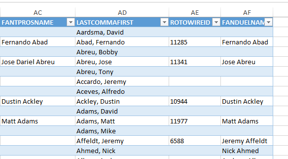
To bring all this data together, I recognized that we need a way to match a player’s name according to FanDuel to the player ID systems shown on the Player ID Map. So I made an update to the map over the weekend and added “FANDUELNAME” in column AF (I also added over 30 new players that have been called up during this season and/or are starting to have a “fantasy impact”. Guys like Carson Smith, Nate Karns, Carlos Frias, Lance McCullers).

If you’re using the Player ID Map and you want instructions on how to drop in an updated version, check this out.

But We Had a Problem

Look closely at the image below.

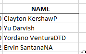
Who the heck is “Clayton KershawP”?

If you look through the list a little more you will see “Jose FernandezDL”, “Yordano VenturaDTD”, and “Ervin SantanaNA”.

You can probably see that some player names are reflecting health or availability information. This is great, but it poses a challenge for our ability to match to the new column in the Player ID Map. Kershaw is going to be listed as “Clayton Kershaw” on the list. Not “KershawP”.

Enter Excel Formulas “RIGHT”, “LEFT”, “FIND”, “LEN”, and “IF”

We are going to use a series of formulas to do the following things:

1. Identify if a player name has “DL”, “DTD”, “NA”, or “P”. I’ve scanned the list of player names and those are the only injury/availability classifications I see.
2. If a player has one of those health indicators on their name we will strip it off
3. If a player does not have health indicators, we’ll just use their name as it is shown

RIGHT

The RIGHT function will give you the rightmost characters in a text string. For example, we could use the RIGHT function to look at the string “Yu DarvishDL” to determine if the two rightmost characters are “DL”.

This formula uses two inputs:

1. Text – The main string of text you want to pull the rightmost characters from (this can be a cell reference)
2. Num_chars – The number of characters to pull out

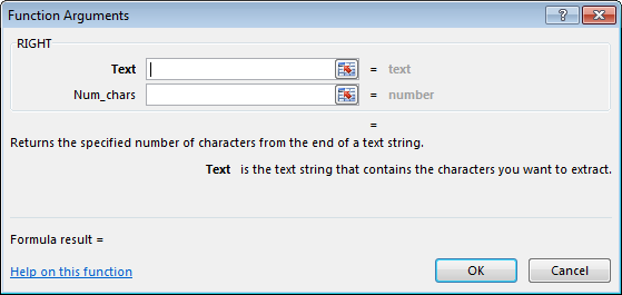
We will use the RIGHT function to look at only the last three characters of each player’s name. We only need the last three because our longest health indicator is “DTD” (three characters in length). And we don’t want to look at full names, because one of our health indicators is just “P”. We can’t just tell Excel to look for a capital P in an entire player name because player’s like Michael Pineda or David Price might cause us trouble. So by limiting our search to just the last three letters in a player name, we should be able to located “DL”, “DTD”, “NA”, and “P” without issue.

FIND

The FIND function searches for a specific string of text within another string of text. If the string you are searching for is located, it returns a number that indicates the location where the string starts. FIND is also case-sensitive (thank goodness, otherwise looking for “NA” at the end of player names could be a problem with guys named “Santana”).

This formula requires two inputs and has one optional input:

1. Find_text – The string of text you are searching for. You can enter your text in double quotes or use a cell reference.
2. Within_text – The string of text you want to search within. This can be a cell reference.
3. Start_num (optional) – What character within the string you want to start searching at. For example, if you wanted to start by searching only after the fifth character in a name, you could enter a five for this argument.

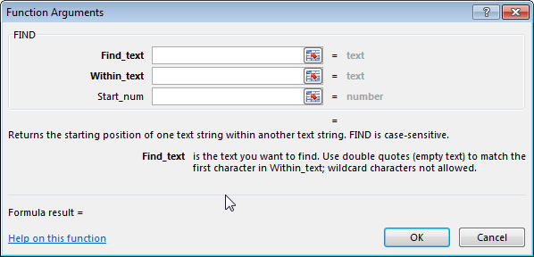
We will use the FIND function in conjunction with the RIGHT formula mentioned above. We will use RIGHT to first pull out only the last three characters from a player’s name. We will then run a FIND on those three characters to look for “P”, “DTD”, “DL”, or “N/A”.

LEFT

Similar to the RIGHT function, LEFT will give you the leftmost characters in a text string.

This formula uses two inputs:

1. Text – The main string of text you want to pull the leftmost characters from (this can be a cell reference)
2. Num_chars – The number of characters to pull out

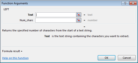
We will use LEFT on players that have health information in their name. For example, for “Clayton KershawP”, we will want to pull out the first 15 characters (out of the total 16 characters in the full string of text).

LEN

The LEN function will tell you the number of characters in a string of text.

This formula has just one input, Text, which represents the text to want to count the characters from. This can be a cell reference.

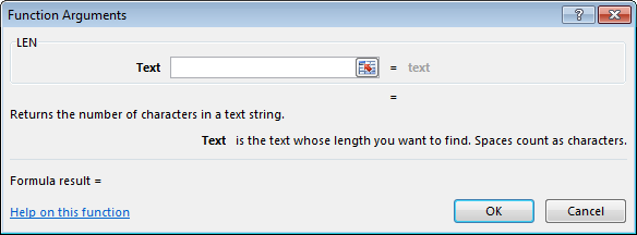
We will use LEN with the LEFT function mentioned above. Remember the “Clayton KershawP” example where I mentioned that string of text has 16 characters and we want to take the leftmost 15 characters? We will use LEN to easily get that 16. We’ll use LEN to evaluate how many characters are in every player’s name.

IF

The IF function allows you to evaluate a cell to see if a condition is true or false. If the condition is true, we can give one result or a specific formula. If the condition is false, we can give a second result or an alternative formula.

This formula uses three inputs:

1. Logical_test – The condition you want to evaluate for being true or false.
2. Value_if_true – The value or formula you want to run if the Logical_test is true.
3. Value_if_false – The value or formula you want to run if the Logical_test is false.

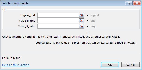
Nesting Formulas

By default, the IF function only allows you two options. One if true. One if false.

This might be a problem for us. Here are some of the tests we need to run…

If we find “P” in the last three characters of the player name, cut off the last character from the name (or if the player’s name is 16 characters in length, give me the leftmost 15). If we find a “DL” in the last three characters of the player name, cut off the last two characters from the name (or give me the leftmost 14 from a 16 character name). If we find a “DTD” in the last three characters, cut off those three letters from the name (or give me the leftmost 13 from a 16 character name). If we find an “NA”, cut off the last two characters (14 from 16). And if none of those are true, then just give me the full length of the player’s name and remove nothing.

Thankfully you can also “nest” IF functions to give you more options. In a weird combination of Excel language and plain English, our formula will look something like this:

This is basically saying, if a player is marked as “P”, cut off one character from their name (that’s what the “-1” is doing in the LEFT(player_name, LEN(player_name)-1). If the player is not marked as “P”, go to the next IF statement. If the player is marked as “DL”, cut off two characters from their name LEFT(player_name, LEN(player_name)-2). If the player is not marked as “DL, go to the next IF statement.

And so on. Until we get to the very end of all the IF statements. The final player_name just indicates that if all the previous IF conditions are false, this is what will show.

One More Web Query Option I Didn’t Mention

We looked at quite a few web query options in the last post, but I neglected to mention one that will now be helpful to use. We are going to be placing the formulas from above next to the FanDuel web query results (you can see my vision of how this will look below, they’re shaded a yellowish color).

The potential problem with doing this is that the web query results and FanDuel’s list of player names will be changing each day and for each contest. The length of the player list is going to be a lot longer for a full slate of games on a Wednesday night than it will be for the afternoon slate on a Thursday.

Fortunately, Excel offers a setting that will attempt to fill the formulas down as far as the data in the web query reaches. To activate this setting, first select a cell in the middle of the web query results (for example, select the cell with Clayton Kerhsaw’s name).

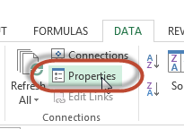
Then click on the “Data” tab. And then click the “Properties” button in the “Connection” section of the Data tab.

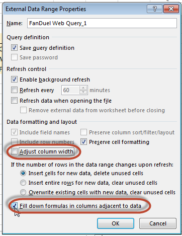
This will bring up the “External Data Range Properties” dialog. Check the bottom check box for “Fill down formulas in columns adjacent to data”. This will attempt to fill our formulas to the exact size of the web query results. I also like to uncheck the “Adjust column width” box because each time the web query runs, it resizes my columns and I find it annoying.

Step-By-Step Instructions

If you want to make sure you’re at the same starting point as me, here’s an Excel file containing the FanDuel Web Query that has the “Fill down formulas…” option already checked. When you open the file in Excel, you will likely have to enable data connections. And then you’ll need to go to FanDuel and identify a contest ID to enter in cell B1.

Step	Description
1.	Before we get into the formulas, enter headers in columns H-L (next to the web query results) for “DL”, “P”, “DTD”, and “NA”. I formatted my column headers bold, I aligned them in the center of the cell, and put a border at the bottom of each cell. We will use the combination of the RIGHT and FIND functions discussed above in the “DL”, “P”, “DTD”, and “NA” columns to detect if a player has any of those statuses in his name. Then the “Name” column will hold our massive IF formula that uses LEFT and LEN to pull out just the player’s name.
2.	Combining multiple Excel functions together can be confusing and lead to errors, so I like to build them up one step at a time. We mentioned earlier in this post that the first step in detecting the availability/health information is to look only at the three rightmost characters in his name. To do this, we’ll use the RIGHT function. Enter the following formulas in the first “DL” cell (H5 in my example file): =RIGHT($B5,3) The reason for the dollar sign is because we will be using the same RIGHT formula in the “P”, “DTD”, and “NA” columns. We want the column to be an absolute and not relative cell reference (if we copy the RIGHT formula to column I, we don’t want it to become =RIGHT(C5,3)). You should be able to see that our formula is working.
3.	Now we will wrap the FIND function around the RIGHT formula we just created. Adjust your existing formula by adding the red text below: =FIND(H$4,RIGHT($B5,3),1) We want to find the string “DL” in the three rightmost characters of Clayton Kershaw’s name and we want to start looking for the “DL” string at the first character. This time we want our row number to be absolute, so the dollar sign goes to the left of the row number. As we copy this formula to column I, we want it to look at the “P”. But as we copy the formula down to other rows we still want it to be locked on row four.
4.	After you complete that formula, you’ll likely have a “#VALUE!” error. This is indicating that the “DL” string was not found in the player name. We need to correct this because our “NAME” column will eventually be referring to this cell and that formula will then also result in an error. To resolve this we will now wrap our existing formula inside one more function: =IFERROR(FIND(H$4,RIGHT($B5,3),1),0)
5.	Select the cell containing your completed formula (cell H5). Copy this formula to the “P”, “DTD”, and “NA” columns by dragging the square in the bottom right hand corner of the cell to those columns. Then double click the same square to copy the formulas to all of the data below.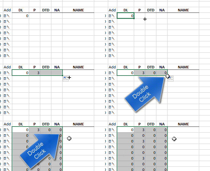
6.	Look closely and verify the results. You should see that anyone with an availability status shows a number greater than 0 in the applicable column, while players with no status show zeroes across all columns.
7.	Put your thinking cap on. Here comes the monster IF formula. Find a player that has a “DL” status. We’ll first start with just getting the LEFT function to work on one player. My first DL’ed player is Yu Darvish in row 22. I’ve hidden some rows in between so you can keep some perspective when looking at the screenshots. Enter the following formula in the appropriate row of the “NAME” column (I’m entering my formula in cell L22, adjust your formula for the row you’re working on): =LEFT(B22,LEN(B22)-2) In this case, the LEN function will determine that “Yu DarvishDL” contains 12 characters (including the space). We then subtract two from that because we know the “DL” is included on the end of the name, meaning we only want the leftmost 10 characters from the string. Moving outward from the LEN function, the LEFT function looks at “Yu DarvishDL” and takes the 10 leftmost characters (the length of 12 minus 2), resulting in just the name “Yu Darvish”.
8.	The LEFT formula we just completed is what we want evaluated if a player is on the DL. To make this happen, we’ll use the LEFT formula as our true condition in an IF function. =IF(H22>0,LEFT(B22,LEN(B22)-2),B22) We know that any player with a health status after their name will have a number greater than 0 in the applicable status column. That’s where the H22>0 logical test comes in. If a player is on the DL, our formula should strip off the “DL” status. But if he’s probable or day-to-day, we should still see those codes. Copy the current formula to all players, in order to see if this is what’s happening.
9.	Now we’ll nest in another IF function to identify “P” players using the same principles we just used in steps 7 and 8. Remember, I’m working in row 22, just because that’s where I started. Adjust the “22” references in my formula to the row you’re working on. =IF(I22>0,LEFT(B22,LEN(B22)-1),IF(H22>0,LEFT(B22,LEN(B22)-2),B22)) The new LEFT formula is identical to the last one except this time we’re subtracting 1 instead of 2. This is because “P” is one character long while “DL” was two. Copy this formula to all players. I’ve just taken our original IF formula and made it the “Value_if_false” argument inside a new IF formula. Now our formula is checking to see if a player is “P” and stripping that status off and if they’re not “P”, it checks to see if they’re “DL” and strips that off, and if neither of those conditions are true, it just takes the full name (so you should still see “DTD” and “NA” players).
10.	Let’s nest another IF function. This time to identify “DTD” players. Remember, I’m on row 22… =IF(J22>0,LEFT(B22,LEN(B22>-3),IF(I22>0,LEFT(B22,LEN(B22)-1),IF(H22>0,LEFT(B22,LEN(B22)-2),B22))) This time we’re looking at column J for “DTD” players and subtracting three characters from the player’s name. Copy this formula to all players. All “P”, “DL”, and “DTD” player names should be correct! “NA” is all that remains.
11.	Last IF function. Row 22 reminder… =IF(K22>0,LEFT(B22,LEN(B22)-2),IF(J22>0,LEFT(B22,LEN(B22)-3),IF(I22>0,LEFT(B22,LEN(B22)-1),IF(H22>0,LEFT(B22,LEN(B22)-2),B22)))) This last time we’re looking at column K for “NA” players and subtracting two characters from the player’s name. Copy this formula to all players.
12.	BAM! Nice work.

Now That We’ve Separated the Men From the Boys

If you’re reading this line of the post, I just want to say thanks. I know the information on this site isn’t for everyone. But at the same time, there are a select few curious and hard working fantasy baseball players wanting to get their hands dirty and to get better at what they do. You’re obviously one of those people and hopefully you’re finding some value in this.

What’s Next

I think we’ll try to bring the FanDuel information from this spreadsheet together with the Player ID Map. Then from there we can bring in outside information like player stats, weather, and opponent data.