I know, I know. It’s mid-March, college basketball is taking over your time, and you’re in the final push of draft preparation for your baseball leagues. The last thing you want to do right now is start tinkering with your draft spreadsheet and screw something up.
Then here I come with another monster Excel post…
NOT THIS TIME! I swear. This is an easy one and you might find it helpful.
In this post I’ll show you how to use Excel’s conditional formatting to gray out players that have been chosen during your draft.
Excel’s Conditional Formatting
Conditional Formatting is a way to adjust the format of individual (or many) cells based upon the information within that cell. If you were using this in a business spreadsheet you might want really high sales months to show up in bolded font or below average sales people to show up shaded in red.
For fantasy baseball you might want all players projected to hit 30 HR to have their HR projection in bold red font. Who knows.
The point is you can tell Excel “what to format” and “how to format it”.
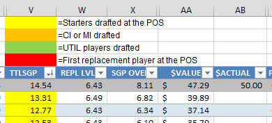
Here’s an example of what I’ll show you in this specific post:
Assumptions
I’m using Excel 2013 in the screenshots below. I think this will work on Excel 2007 or 2010 without any issues. I’m also assuming you’re starting with a spreadsheet you created following either this standings gain points series or this points league series.
Step-by-Step Instructions
| Step | Description |
|---|---|
| 1. | The first thing you need to do is decide how you will track drafted players. You could use the method I’ve described here. Or if you’re in an auction you could track who has been drafted simply by putting the dollar value each player was sold at in the $ACTUAL column of your spreadsheet.
It doesn’t matter what method you choose, but for this example I’m going to assume that whatever column you use to track will be blank if the player has not been drafted and there will be some value in the column if the player has been chosen. Make note of the column number of your choice. For example, I’ll be using column “AB” based on the image below. |
| 2. | Click on the first player ID in column A of your “Hitter Ranks” tab. Then hit CTRL + SHIFT + END (all at the same time) to select the remaining rows and columns in the table (Excel should highlight all players and columns).
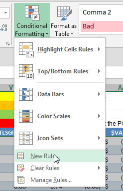
Then on the “Home” tab of the ribbon, click the “Conditional Formatting” drop down and choose “New Rule…”. |
| 3. | In the “New Formatting Rule” dialog that pops up, select the last option of “Use a formula to determine which cells to format”.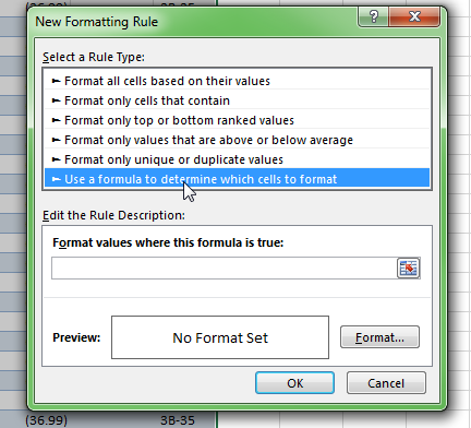 |
| 4. | In the “Format values where this formula is true:” box, enter the following formula
The reason I’m using cell AB6 in this formula is because my $ACTUAL column is where I’ll be tracking who’s been drafted (and that’s column AB). The reason row 6 is referenced is because I added some information above my table to help define where players a slotting for determining replacement level (whether they’re a starter, falling to MI or CI, UTIL, etc.). My first player doesn’t appear in the sheet until the sixth row. A few things to keep in mind about this formula. The equals sign at the beginning is very important. Excel will let you get away without typing in the equals sign but then the formula will not work properly. In plain English, the The dollar sign before cell “AB6” is to tell Excel, “Only look in column AB for the blank cells”. If we left the dollar sign out Excel would start shading seemingly random areas. If you get to the end of this set of instructions and you have weird shading showing up, check this again. |
| 5. | Now that we’ve given the instructions on what to shade, let’s decide how to shade these drafted players. Click the “Format…” button. |
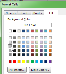
| 6. | You can format a variety of things for each cell (although some options gray out when you have a large block of cells selected like we do). The “Fill” tab will allow you to shade cells a certain color.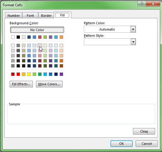
I’m going to shade drafted players gray. After you’ve chosen your color click “OK” to accept your color choice and then “OK” to accept the conditional formatting rule (we’re done setting up the rule now). |
| 7. | If you have not entered any auction values or that any players have been selected, nothing will be shaded yet. To test that everything is working, add a dollar value to the “$ACTUAL” column or enter a team name in the “LGTEAM” column (from this example). |
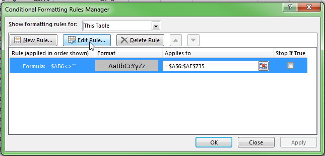
| 8. | If you get to the end and you find out the formatting is not working properly, you can edit the rule by going to the “Manage Rules” drop down option under the “Conditional Formatting” menu on the ribbon.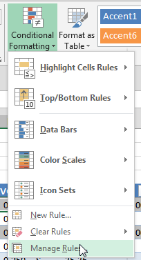
Then select your rule and click the “Edit Rule…” button. |
Think of What Else is Possible
Conditional Formatting in Excel is something a lot of people don’t know about and even those that do know it exists can find it intimidating. It can be confusing to work with, but if you follow the principles outlined above, you’ll be able to do some really neat things.
I’ve only given you one small practical way to use this. But there are A LOT of other neat things you could do with this.
Want to shade all outfielders a certain color? Or highlight all players with multiple position eligibility? How about tell the difference between a starter and a reliever? Left-handed hitters versus righties? Shade all injured players red so you don’t draft them?
Have Questions?
Please ask me any questions you have about this in the comments area at the end of this post.
Want to Know How to Do Something in Excel?
If you have a suggestion or question on how to do something fantasy baseball related in Excel, shoot me an e-mail at smartfantasybaseball at gmail dot com.
Want More Info Like This?
The best way to stay in touch with the site and to get more information like this is to follow me on Twitter or to register as an SFBB Insider.







i followed directions but it is shading the row above the intended row — any thoughts?
I’d double check that your first player starts in Row 6, and if they don’t, adjust accordingly. Also make sure the “Applies To” range starts on the same row as your first player. For example, the rule I applied is =$AB6″” and the “Applies To” range starts on row six too ($A$6:$AE$735). Could you have one starting on row 5 and one on row 6?
Hi Tanner,
I took it a different way, and let me know if this is totally wrong. In drafts I notice that sometimes I need to draft somebody who is better at something specific. I.E. based on my keepers for this year I know I need to make up ground in HR and AVG. So for each of the 5 categories, I conditionally formatted each players SGP based on the 168 player pool. I colored players Red if they were 3 standard deviations above the average (very few of those across all categories) colored them orange if they were 2 standard deviations above, green for one and blue if they are above average. Now I can sort by colors to look at the remaining players that will help me in AVG, or quickly look and see that, yes sure enough Altuve is red in avg, he will really help me there, but he is below average in HR. Is this viable by using their SGPs per category or should I go straight to the counting stats? Thanks so much for all your work!
Hi Chris,
Thanks for reading the site and for sharing your ideas.
I don’t think it matters much. Just be sure you understand what you’re looking at. If you follow the process I outline in my SGP book exactly, those SGP numbers can be considered SGP above replacement level. That could be a little deceiving if the replacement level players are “specialists” of some kind (e.g. speedy players or high power low average guys). If it’s raw SGP vs. raw counting stats, I don’t think it should matter.
Thanks, Tanner
Tanner, thanks for all the awesome tools. I’m in my infancy of using excel to build rankings, cheat sheet, etc. I think with more time next year I’ll get into building my own projections (where the real “fun” is). One question regarding conditional formatting. I had no problem creating a dark grade shade to block out drafted players once I selected a team from the drop down list on my “rankings page”. Any idea how can I apply the same conditional formatting to the cheat sheet I created to simultaneously shade out the same guys? Hope that makes sense.
Hi Steve,
I think you would need to put a column next to each position. In that column you would do a VLOOKUP (or INDEX/MATCH) to see if the player was drafted. Use the VLOOKUP to pull back the team the player was drafted by. Then set up the conditional formatting to shade if the cell is not blank.
I realize this is ultra brief. But I’ll consider a more detailed version in the future.
Tanner
That’s what I had setup, but was hoping maybe you had something I wouldn’t see. Not that big of deal. Thanks for getting back to me so quickly.