Welcome to the first part of a series in which we’ll go step-by-step through the process of using Microsoft Excel to calculate your own rankings for a fantasy baseball points league (as opposed to rotisserie or head-to-head rotisserie).
Whether you’re in a standard points league at a major site like ESPN or a more advanced Ottoneu league at Fangraphs, this process will help you develop customized rankings for your league. These instructions can be used for a season-long points league or a weekly head-to-head points league.
If you’re looking for info on how to rank players for a roto league, look here.
I recommend going through all the parts of the series in order. If you missed an earlier part of this series, you can find it here:
ABOUT THESE INSTRUCTIONS
- The projections used in this series are the Steamer 2015 preseason projections from Fangraphs. If you see projections that you disagree with or that appear unusual, it’s likely because I began writing this series in December 2014, still early in the off-season.
- For optimal results, you will want to be on Excel 2007 or higher. Some of the features used were not in existence in older versions.
- I use Excel 2013 for the screenshots included in the instructions. There may be some subtle differences between Excel 2007, 2010, and 2013.
- I can’t guarantee that all of formulas used in this series will work in Excel for Mac computers. I apologize for this. I don’t understand why Excel operates differently and has different features on different platforms.
IN PART 5
In this part of the series we will use the named cells created in Part 2 along with our projection information on the “Hitter Ranks” and “Pitcher Ranks” sheets to calculate total projected points for each hitter and pitcher.
Please note that this series has been adapted into a nine-part book that also shows you how to convert points over replacement into dollar values and how to calculate in-draft inflation. Click here if you’re interested in reading more about the conversion to dollar values.
EXCEL FUNCTIONS AND FORMULAS IN THIS POST
We’ll just be doing some basic addition and multiplication. We won’t be adding in any new features, but we will be doing this basic math using the named cells for your league’s scoring settings that we created in earlier parts of the series. 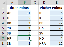 To refresh your memory and to see the complete list of named cells, access the “Formulas” tab of the Ribbon and then click the “Name Manager” button.
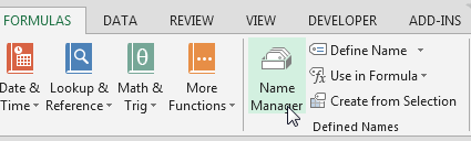
The list will display all named cells/ranges and named tables. To view only named cells, click on the “Filter” drop down menu and choose “Defined Names”.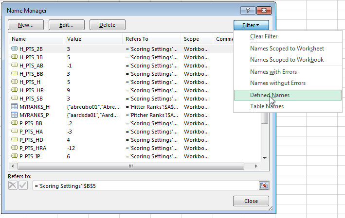
STEP-BY-STEP INSTRUCTIONS
| Step | Description |
|---|---|
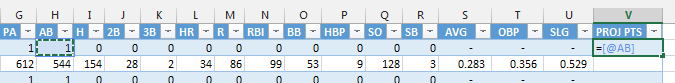
| 1. | Go to the “Hitter Ranks” tab in the Excel file.In the first open column next to the table data (e.g. cell V1), type in “PROJ PTS” as the column header. Excel should expand the table to include this new column.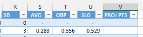 |
| 2. | Recall from looking at our named cells above that we named our hitting point values using a “H_PTS_” prefix followed by the abbreviation for the statcategory.In my example league, the hitting point values have the following names in Excel:
Follow the steps below using the scoring categories and named cells that you set up. Follow these steps with your league in mind. We’ll now use those names to build a formula to calculate projected points. In my example league, the first hitting scoring category is At Bats (H_PTS_AB). In the first empty cell below the “PROJ PTS” header (e.g. cell V2), type an “=” and then click on the corresponding stat for the player in this row. My first player is Bobby Abreu (wow!). So I clicked in cell H2, the projected ABs for Abreu. |
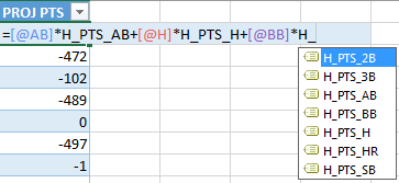
| 3. | While still editing this formula we’ve started, we must now multiply the projected AB for Bobby Abreu by the point value for AB.Type the sign for multiplication (the *, or SHIFT + 8). Then begin to type “H_PTS_”.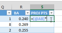 Excel should recognize the name you’re typing and present you with a list of named cells which follow that pattern. Once you see this list you can double-click on the desired name, use your arrow keys to select “H_PTS_AB” and hit TAB to choose it, or just continue typing the full name. Excel should recognize the name you’re typing and present you with a list of named cells which follow that pattern. Once you see this list you can double-click on the desired name, use your arrow keys to select “H_PTS_AB” and hit TAB to choose it, or just continue typing the full name.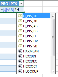 In my scoring system, I want “H_PTS_AB”. Hit enter to save the formula at this point.My completed formula at this point is: In my scoring system, I want “H_PTS_AB”. Hit enter to save the formula at this point.My completed formula at this point is:
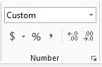
You may need to use the “Number” format options on the “Home” tab of Excel’s menu system to adjust the appearance of your points. |
| 4. | Review the output of the “PROJ PTS” column at this point to make sure it seems to be working correctly.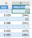 The league I play in has an unusual scoring system that penalizes for outs (just like in real baseball, an out is a bad thing). That’s where the negative value for an AB comes in. The league I play in has an unusual scoring system that penalizes for outs (just like in real baseball, an out is a bad thing). That’s where the negative value for an AB comes in. |
| 5. | Repeat steps 2, 3, and 4 above in order to add in the other hitting scoring categories of your league. Just begin at the end of your original “PROJ PTS” formula, add a “+” sign, and add in the next scoring category and point value.It may be a good idea to build the formula one stat category at a time so that you can do a quick reasonableness check.
For example, building on the formula I started above, to add points for hits, I would edit my “PROJ PTS” formula to be:
Continue until you have added in the points for each category.
|
| 6. | The accountant in me really really wants you to double check the formula you just created.
Make sure it seems consistent and that the [@AB] argument is paired with “H_PTS_AB”, and all other categories align with their point value name).After all, it probably only took you a couple of minutes to create this formula. It will probably only take another 30 seconds to review it closely… And your WHOLE fantasy season depends on it! |
| 7. |
If the formula looks good, you can give it one more great check by sorting the “Hitter Ranks” tab by “PROJ PTS” to see who the best players are. To do this, click the downward pointing filter arrow on the “PROJ PTS” column. Then click on “Sort Largest to Smallest”. |
| 8. | Go to the “Pitcher Ranks” tab in the Excel file. In the first open column next to the table data (e.g. cell S1), type in “PROJ PTS” as the column header. Excel should expand to include this new row.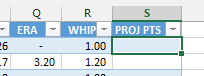 Recall that we named our pitching point values using a “P_PTS_” prefix followed by the abbreviation for the stat category.In my example league, the pitching point values have the following names in Excel: Recall that we named our pitching point values using a “P_PTS_” prefix followed by the abbreviation for the stat category.In my example league, the pitching point values have the following names in Excel:
Follow the steps below using the scoring categories and named cells that you set up. Follow these steps with your league in mind. |
| 9. | Let’s start to build a formula to calculate projected pitching points, starting with the first pitching point category.
In my example, the first pitching category is Innings Pitched (P_PTS_IP).In the first empty cell in the “PROJ PTS” (e.g. S2), type an “=” and then click on the corresponding stat for the player in this row. My first player is David Aardsma (who at one point in time had fantasy-relevance, so he made it into the PLAYERIDMAP). To include Aardsma’s IP, I clicked in cell J2 (remember, your columns may be slightly different depending on when you and where you downloaded your projection data from). |
| 10. | While still editing this formula we’ve started, we must now multiply the projected IP for Aardsma by the point value for IP.
Type the sign for multiplication (the *, or SHIFT + 8). Then begin to type “P_PTS_”.
You may need to use the “Number” format options on the “Home” tab of Excel’s menu system to adjust the appearance of your points. |
| 11. | Review the output of the “PROJ PTS” column at this point to make sure it seems to be working correctly.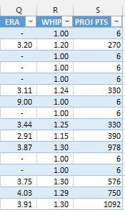 |
| 12. | Repeat steps 9, 10, and 11 above in order to add in the other pitching scoring categories of your league. Just begin at the end of your original “PROJ PTS” formula, add a “+” sign, and add in the next scoring category and point value.It may be a good idea to build the formula one stat category at a time so that you can do a quick reasonableness check.
For example, building on the formula I started above, to add points for strike outs, I edit my “PROJ PTS” formula to be:
Continue until you have added in the points for each category.
You might have noticed that my league’s scoring system uses Holds as a pitching category but I’ve neglected to include that in my formula. I have not been able to find a reliable projection system that projects Holds, so I’ve just ignored it. I have no research to back this up, but I feel I can largely ignore Holds during the draft. By studying team depth charts and watching bullpen usage early in the season, I think I’ll be able to identify unexpected sources of Holds during the season. |
| 13. | The entire quality of your draft depends on this formula.
Double check the consistency of your formula (check that the [@IP] argument is paired with “P_PTS_IP”, and all other categories align with their point value name). |
| 14. |
If the formula looks good, you can give it one more great check by sorting the “Pitcher Ranks” tab by “PROJ PTS” to see who the best players are. To do this, click the downward pointing filter arrow on the “PROJ PTS” column. Then click on “Sort Largest to Smallest”. |
| 15. | Save your file. |
 My final formula is:
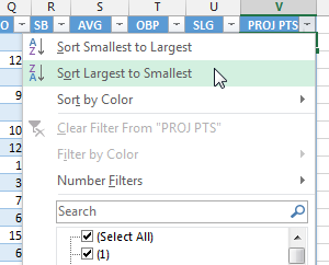 Hopefully you’ll find that the players come out in an order that seems appropriate given your scoring system (does Mike Trout come out near the top?).
 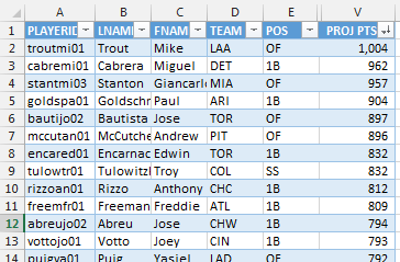 Now let’s move on to the pitchers.
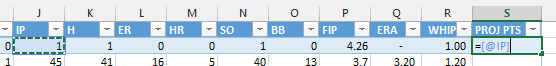
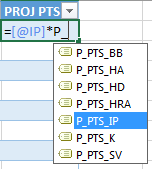 In my scoring system, I want “P_PTS_IP”. Hit enter to save the formula at this point.My completed formula at this point is:
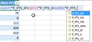 My final formula is:
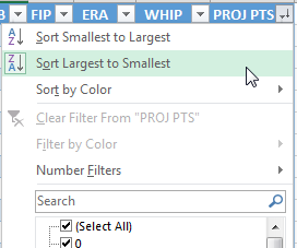 Hopefully you’ll find that the players come out in an order that seems appropriate given your scoring system (does Clayton Kershaw come out near the top?).
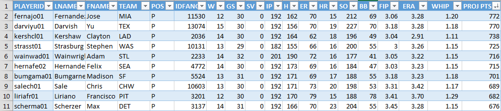
WRAP UP
We now have total projected points for both hitters and pitchers, and you might be wondering, “What else is left to do?”.
In our next part of the series we’ll add the important adjustment for replacement level. Failing to incorporate replacement level into your calculations can lead to some poor decisions. You can check out part six here or see all parts of the series in one place If you have questions, it would be great if you can ask them in the comments below so others can benefit from the discussion.
If you’d like to know when I put out the next post in the series or similar posts in the future, click below to follow me on Twitter.
Do you have any questions about Part 5? Please leave them here and I’ll do my best to answer them.
Can you pull the data from Hitter’s Rank and Pitcher’s Rank into one table so you can have a complete all inclusive list?
Hi Dan, I don’t have a very elegant way to do this, but this seems to work.
='Hitter Ranks'!A6(this should correspond to the very first ID of the very first hitter listed on the Hitter Ranks tab).=IFERROR(VLOOKUP(A2,MYRANKS_H,COLUMN(MYRANKS_H[$VALUE]),FALSE),0)='Pitcher Ranks'!A2(again, this should correspond to the very first ID of the first pitcher on the Pitcher Ranks tab).=IFERROR(VLOOKUP(A801,MYRANKS_P,COLUMN(MYRANKS_P[$VALUE]),FALSE),0)Hope that helps.
Tanner
For some reason the stats don’t show up for some players like Mike trout in the hitters rankings.
I probably put something where it shouldn’t, IDK.
Thanks
Hi Roger,
I’ll e-mail you. I think I may need to look at your file to help troubleshoot better.
Thanks,
Tanner
Hey Tanner,
Loving this tool so far. Extremely helpful to give a leg up on the guys in my league who i am positive are not doing anything like this.
My question is that my pionts league awards a point for total bases. Is there a way I can use the fangraphs projections to figure total bases?
Thanks,
Chris
Hi Chris,
Thanks! I agree, thinking through projections and rankings like this is a huge advantage on many levels.
I think the formula for total bases would be =1*HITS+1*2B+2*3B+3*HR
I know that looks a bit odd, but if you assume one base for each hit, then you’d only add one more base for a double (for a total of two bases). Or a home run would be one base for the hit, then three more for the “extra bases”, for a total of four bases.
To do this, I think you’d pull H, 2B, 3B, and HR from the projections onto the Hitter Rankings tab. Then add a column to calculate total bases using that formula from above. Then add a column for determining the point value you get from the total bases.
Hope that helps.
Tanner