Welcome to the first part of a series in which we’ll go step-by-step through the process of using Microsoft Excel to calculate your own rankings for a fantasy baseball points league (as opposed to rotisserie or head-to-head rotisserie).
Whether you’re in a standard points league at a major site like ESPN or a more advanced Ottoneu league at Fangraphs, this process will help you develop customized rankings for your league. These instructions can be used for a season-long points league or a weekly head-to-head points league.
If you’re looking for info on how to rank players for a roto league, look here.
I recommend going through all the parts of the series in order. If you missed the beginning of this series, you can the earlier parts here:
ABOUT THESE INSTRUCTIONS
- The projections used in this series are the Steamer 2015 preseason projections from Fangraphs. If you see projections that you disagree with or that appear unusual, it’s likely because I began writing this series in December 2014, still early in the off-season.
- For optimal results, you will want to be on Excel 2007 or higher. Some of the features used were not in existence in older versions.
- I use Excel 2013 for the screenshots included in the instructions. There may be some subtle differences between Excel 2007, 2010, and 2013.
- I can’t guarantee that all of formulas used in this series will work in Excel for Mac computers. I apologize for this. I don’t understand why Excel operates differently and has different features on different platforms.
IN PART 4
In this part of the series we will again use Excel’s VLOOKUP and IFERROR formulas as well as Table and Structured Reference features, but this time to pull pitcher information and projections to create our pitcher rankings tab.
EXCEL FUNCTIONS AND FORMULAS IN THIS POST
This is where I normally give detailed explanations of each Excel feature and formula used in the instructions below; however, we’re not introducing anything new in Part 4. If you would like more background on the features and formulas used below, please refer to Part 3 or ask questions in the comments area below.
STEP-BY-STEP INSTRUCTIONS
| Step | Description |
|---|---|
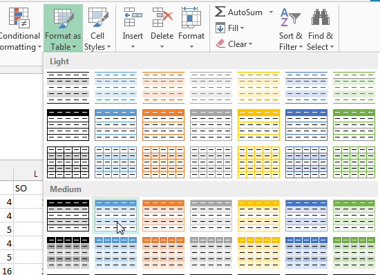
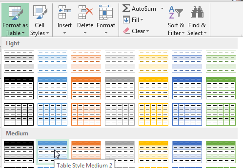
| 1. | Go to the “Steamer Pitchers” tab of your Excel file.We will convert this to a “table” in Excel in order to make the data easier to work with.Click anywhere within the pitcher projection data. Then locate the “Home” tab in the Excel menu system (“the ribbon”).
Click once on the “Format as Table” drop down, and then select your desired color scheme. You might notice that my example projection data goes out to column T. Yours may have more or less columns. I believe the Steamer downloads contain additional information at certain times of the year, but if you look closely at the information in the rightmost columns, they’re things we don’t care about for fantasy (WAR calculations, etc.). As long as you have the main pitching categories needed for your league’s scoring system and the “PLAYERID” column, you’re good.
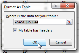
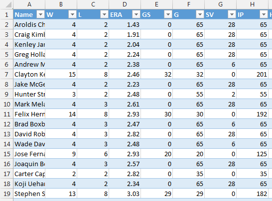
Check “My table has headers”. Click OK. After accepting this, your bland looking data will transform into a nicely formatted table. |
| 2. | We’ll later be pulling information from this table into other worksheets. To make the pulling of data easier we need to move the Fangraphs player ID to be the first column (you can use VLOOKUP if the player ID is in the first column, otherwise you’re stuck using more difficult and/or multiple formulas). Right-click on the top of the Fangraphs player ID column (I right-clicked on the “T” column header) and Cut it.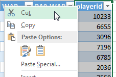 |
| 3. | Now right-click on the top of the player name column (column header “A”) and select “Insert Cut Cells”.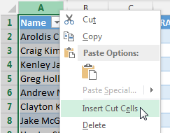 |
| 4. | Before we finalize this table, we should give it a name we can refer to in the future. Go to the “Formulas” tab on the Excel ribbon and click on the “Name Manager” button. |
| 5. | Because we created named cells in Part 2 of the series, it can be difficult to locate the tables in the Name Manager. I find it helpful to filter the Name Manager to only show table names. Do this by clicking the “Filter” drop down menu in the top right of the window. Then choose “Table Names”.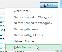 Excel will give very generic names to a table, like “Table2″. It’s more helpful to give meaningful names to your tables. As you get more tables in a spreadsheet, it can become very difficult to remember the difference between “Table2″ and “Table3″.Select your table from the list (it should be the only one named “Table#”) and click on the “Edit…” button. Excel will give very generic names to a table, like “Table2″. It’s more helpful to give meaningful names to your tables. As you get more tables in a spreadsheet, it can become very difficult to remember the difference between “Table2″ and “Table3″.Select your table from the list (it should be the only one named “Table#”) and click on the “Edit…” button. |
| 6. | Give the table a meaningful name. I chose “STEAMER_P” to indicate these are the Steamer Pitcher projections.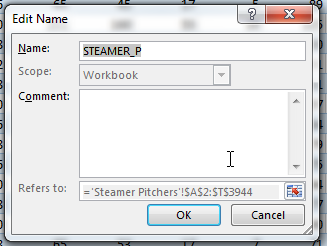 Click “OK” to close the “Edit Name” menu. Then click “Close” to exit the “Name Manager”. Click “OK” to close the “Edit Name” menu. Then click “Close” to exit the “Name Manager”. |
| 7. | We now have two tables ready to pull pitcher information from, PLAYERIDMAP and STEAMER_P.I’m going to pull from these two tables into a new tab where I’ll calculate the pitcher rankings. |
| 8. | Right click on the “PLAYERIDMAP” tab and select the option to “Insert…”. 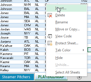 Choose the “Worksheet” option and click “OK”. Choose the “Worksheet” option and click “OK”. 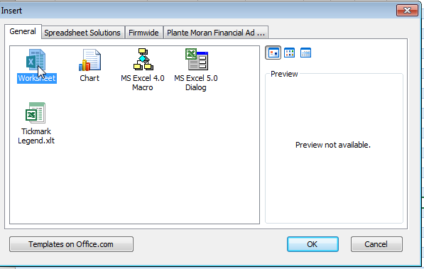 |
| 9. | Right click on the new sheet tab and choose to “Rename”. I’ll call this sheet “Pitcher Ranks”.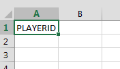 |
| 10. | As we have talked about before, I like to use Baseball-Reference player IDs as the main ID system in my spreadsheets. This is so I can look at an ID and know who the player is (e.g. kershcl01 is Clayton Kershaw). To make it the main ID we want the first column of this new sheet to contain the Baseball Reference player ID and we only want pitchers at this time. The PLAYERIDMAP sheet has a list of all fantasy-relevant players (for standard rotisserie leagues, at least) and their Baseball Reference IDs. However, this sheet contains hitters also. Because this sheet is an Excel table, it’s easy to filter out those hitters. Click on the drop down arrow on the “POS” column. You’ll be presented with a list of all the positions. Check the “(Select All)” box until all the positions below become unchecked. Then check the “P” box. Click OK to apply the filter.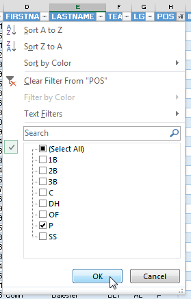 The Player ID Map will now list only pitchers. The Player ID Map will now list only pitchers. |
| 11. | Starting at the first player and ending with the last, click and drag within the “IDPLAYER” column (first column) and select all player (or select the first player and then use the keyboard shortcut SHIFT + CTRL + Down Arrow). Only select from this first column. |
| 12. | Copy this selected data. Return to the “Pitcher Ranks” sheet. Then paste the data into cell A2.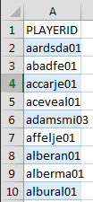 |
| 13. | Now that we’re starting this new sheet, we should convert it to an Excel table. We will essentially repeat step 1 above, but for this new worksheet.
Click once to select any player ID. Then locate the “Home” tab in the Excel menu system (“the ribbon”). Click once on the “Format as Table” drop down, and then select your desired color scheme. |
| 14. | You will then be prompted to verify the range of cells in the table and that your table has a header row. 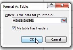 Check “My table has headers”. Click OK. Check “My table has headers”. Click OK. |
| 15. | Repeat steps 4-6 in order to give the table a more meaningful name. In my example, Excel defaulted the table name to “Table6″. I renamed mine to be “MYRANKS_P” (to indicate pitcher ranks, because we already ranked hitters).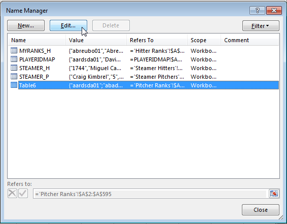 |
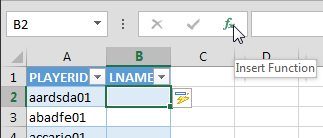
| 16. | Now let’s begin pulling data from the other tabs. I’ll first add “Player Last Name” to the table. To expand your table, simply type into column B and hit Enter (I typed into cell B1). Excel should automatically pull this new column into your table. I’m going to name my column “LNAME”.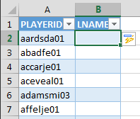 |
| 17. | Your table shading may look like this instead of the image from step 16: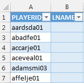 If so, click once in the area between the Column “A” header and the Row “1” header (the top left corner of all cells), to select all cells in the entire sheet. If so, click once in the area between the Column “A” header and the Row “1” header (the top left corner of all cells), to select all cells in the entire sheet.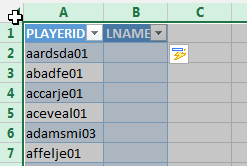 Then click the “Fill Color” icon (looks like a paint can) drop down arrow and choose the “No Fill” option. Then click the “Fill Color” icon (looks like a paint can) drop down arrow and choose the “No Fill” option.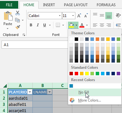 You should now see the proper alternating color scheme. You should now see the proper alternating color scheme.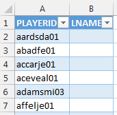 |
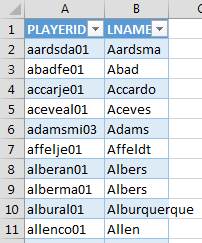
| 18. | Our goal in this column is to instruct Excel to take the PLAYERID from column A, go into the first column of PLAYERIDMAP, find the matching PLAYERID, and then pull the corresponding LASTNAME. You can see in the image of the PLAYERIDMAP below that LASTNAME is in the fifth column (column E).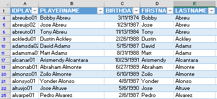
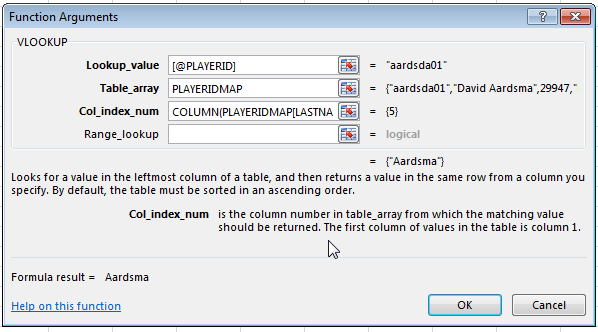
To start building the formula, click in cell B2 of your Pitcher Ranks tab. Then click the “fx” button of the formula bar to launch Excel’s formula wizard. We’ll use the wizard the first time through to better explain this function in Excel. |
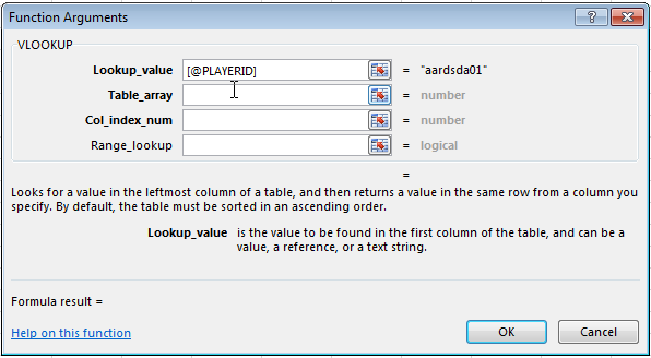
| 19. | Type “vlookup” into the search bar and click “Go”. When the function appears, make sure it is selected and hit “OK”. You should then see the different arguments, or components, needed for the formula to work. 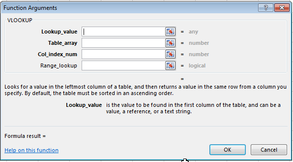 |
| 20. | The “Lookup_value” is the value on the “Pitcher Ranks” sheet that we want to locate (or match to) in the “PLAYERIDMAP”.
Click once in the “Lookup_value” field. Then click on the value in cell A2 (“aardsda01″). Excel will convert this to [@PLAYERID]. As we talked about in Part 3, this naming convention is referred to as a “Structured Reference” or a “Table Reference” and can be used when you have converted your data into an Excel table. |
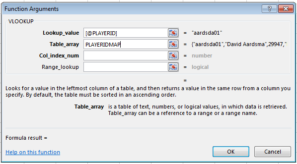
| 21. | The “Table_array” field is the table (or array, or block of data) in which to go look for the matching PLAYERID. Because the PLAYERIDMAP sheet was previously set up as a table, we can take advantage of this.
Click once in the “Table_array” field. Simply type “PLAYERIDMAP” (no quotes). You’ll know you got this right if you see part of the PLAYERIDMAP populating to the right of the Table_array field.
|
| 22. | The “Col_index_num” field wants to know the number of the column in the PLAYERID map table to retrieve data from.
Again, our goal is to retrieve LASTNAME from the PLAYERIDMAP table, which is column 5 in that table. You could manually flip back and forth between tabs to determine the column number. You could then enter a “5” in for “Col_index_num”. This takes time and can be difficult if you start getting into column X (do you know what number letter of the alphabet that is?). It’s also a problem if you later add a column that would push LASTNAME into column number 6. For these reasons, I prefer to use the COLUMN formula. When this is entered into the Col_index_num field, it will calculate the location of the LASTNAME column. We don’t have to flip back and forth. And if LASTNAME gets shifted to another column, this formula will adjust automatically. The formula below will determine that LASTNAME is the fifth column in the PLAYERIDMAP table.
Enter this equation into the Col_index_num field. |
| 23. | Finally, we have the Range_lookup argument. I always enter “FALSE” for this in order to ensure Excel only locates exact matches for a PLAYERID. I don’t want Excel to return an approximate match if the exact PLAYERID cannot be found.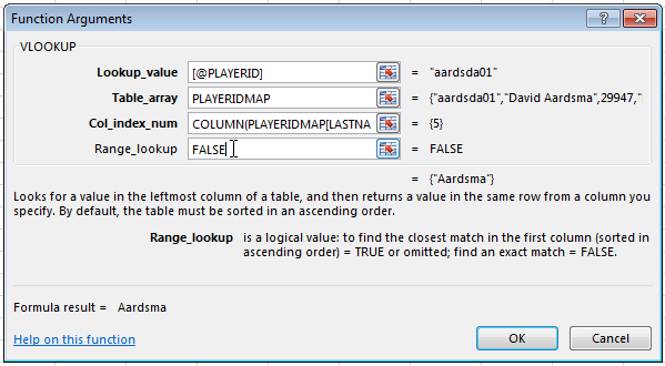 |
| 24. | Before hitting “OK” to accept the formula, you can preview the output. In this case we are dealing with “aardsda01″, or David Aardsma (fantasy stud), and can see the formula appears to be working (you can see the end result of this formula is {“Aardsma”}.
Click OK to accept the formula. Once the formula is entered, it should automatically copy to the remaining rows of the table. |
| 25. | We will use the VLOOKUP formula to pull additional data, and the majority of the formula will remain the same. To add a FNAME column, type the “FNAME” into cell C1. Copy the formula from cell B2.Don’t click and drag it. Actually right-click on B2 to copy it or use the CTRL + C shortcut. Paste the formula into cell C2. When you copy and paste the formula this way you should end up with two columns displaying player last names. That’s what you want for now!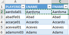 Then simply double click in cell C2 and change the column name (remember column names are surrounded in [brackets]. So change [LASTNAME] to [FIRSTNAME].). Then simply double click in cell C2 and change the column name (remember column names are surrounded in [brackets]. So change [LASTNAME] to [FIRSTNAME].). Nerdy Excel talk here, but dragging formulas within tables does not work very well because there’s no way to make the formulas absolute (they want to stay relative as you move them). That’s why I suggest copying and pasting the formula, even if it duplicates and you then need to change part of it. Nerdy Excel talk here, but dragging formulas within tables does not work very well because there’s no way to make the formulas absolute (they want to stay relative as you move them). That’s why I suggest copying and pasting the formula, even if it duplicates and you then need to change part of it. |
| 26. | Repeat step 25 to pull TEAM, POS, and IDFANGRAPHS from the PLAYERIDMAP tab.
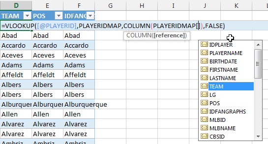
If you can’t remember the exact name of a column, once you have entered a table name, like PLAYERIDMAP, and the opening “[” bracket, a helpful type ahead box will display all the column names in the PLAYERIDMAP table. You can use the mouse to double-click on the column name in the type ahead list or select a column name and hit the Tab key to add it to your formula. The exact formulas you want are: TEAM:
POS:
IDFANGRAPHS:
|
| 27. | We’ve now pulled all the relevant information fromPLAYERIDMAP and can now begin pulling in pitcher projections from our STEAMER_P table.
Add column headers for where we can pull wins (W), games started (GS), saves (SV), innings pitched (IP), hits (H), earned runs (ER), home runs (HR), strikeouts (SO), walks (BB), fielding independent pitching (FIP), and any other counting stat categories used in your league’s scoring system (e.g. L). There will be some tweaks to the VLOOKUP formula we used earlier. First, the Steamer projections use Fangraphs ID numbers. So we will be using the IDFANGRAPHS column as the Lookup_value. Second, we must specify to pull from the Steamer Pitchers projections (STEAMER_P table name). And finally, the COLUMN formula will change to determine what statistic to pull Your final Wins formula should be:
|
| 28. | After you accept the formula above, you may encounter a situation where the VLOOKUP formula will return “#N/A” for certain players.This error means that Excel could not find the value you told it to look up. In this example image below, Chris Carpenter’s player ID was not found in the projections (probably because he’s retired).
These errors can cause big problems with the rankings. It would be better to have the W, ER, and SO’s for a player to be zero or blank. To accomplish this, we can use the “IFERROR” formula and wrap it around our original formula. This is the original formula in the cell: =VLOOKUP([@IDFANGRAPHS],STEAMER_P, Now surround the VLOOKUP formula with the IFERROR formula. The original VLOOKUP formula will remain exactly as is. I will just put “IFERROR(” in front of it. And behind the existing formula I will put “,0)”. =IFERROR(VLOOKUP([@IDFANGRAPHS],STEAMER_P, You can see the edits I made in the red bolded font. That’s all you have to do. Excel will now perform the exact same calculation as before, but if a player cannot be located in the VLOOKUP, Excel will put 0 instead of #N/A. I recommend using a 0, but if you want it to be a blank instead of a zero, use this: =IFERROR(VLOOKUP([@IDFANGRAPHS],STEAMER_P, |
| 29. | The formulas for GS, SV, IP, H, ER, HR, SO, BB, andFIPare shown below.GS:
SV:
IP:
H:
ER:
HR:
SO:
BB:
FIP:
|
| 30. | I don’t pull ERA or other rate statistics, like WHIP, directly from the projections. I prefer to recalculate them with a formula after the underlying statistics have been pulled.
To do this, type “ERA” in as the next column header. Then enter the formula to calculate ERA (=([@ER]*9)/[@IP]).
If you’re not exactly sure of the convention for the formulas (with the brackets and @ symbols) you can always use your mouse to click on the values in the “ER” and “IP” columns and Excel will translate it into the =(@ER]*9)/[@IP] format for you. Repeat this step to add WHIP and any other rate statistics you desire (K/9, K/BB, B/9, etc.). You might notice that these rate formulas can also result in errors if a player does not have a projection (dividing by 0 causes an error). You can use the IFERROR formula around the calculation to clean this up. Here are the formulas I use for ERA and WHIP: ERA:
WHIP:
|
| 31. | Most statistics don’t need formatting, but ERA and WHIP will. In my file, ERA is located in column “Q”. Click on the “Q” column label (or whatever column ERA is in for you) to select the entire ERA column. Then on the Home tab of the ribbon, click on the comma number format.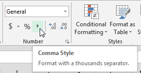 Repeat this same step for WHIP (column R in my example file). Repeat this same step for WHIP (column R in my example file). |
| 32. | Save the file.
You’ve now successfully combined pitcher information and projected pitching stats into one table. |
WRAP UP
We have now completed setting up our hitter and pitcher worksheets that will be used to rank those players and we also have our league scoring settings set up.
In the next part of the series we’ll pull the scoring settings to the rankings sheets and calculate projected points for each player. You can check out part five here or see all parts of the series in one place here.
DO YOU HAVE ANY QUESTIONS?
If you have questions, it would be great if you can ask them in the comments below so others can benefit from the discussion.
If you’d like to know when I put out the next post in the series or similar posts in the future, click below to follow me on Twitter.

 You will then be prompted to verify the range of cells in the table and that your table has a header row (e.g. Name, W, L, ERA, etc.).







Will you explain how to import Holds and HRs Allowed for Ottoneu players?
Hi Rich,
HRs are included above (I just labelled them HR not HRA). But Holds are a difficult topic. Steamer does not project Holds. I don’t think any of the Fangraphs projection systems do. If you do know of a source that projects Holds let me know and I can try to create something for it. Feel free to e-mail me.
Worst case scenario, you could go back to the earlier parts in this series and create a scoring cell for Holds, then add a column for Holds to the “Pitcher Ranks” tab, and then put in your own estimates/projections for players.
Hope that helps some,
Tanner
CBS projects holds
Thanks, Jason. I’ll look into that.
Jason, do you have a link to a CBS page that displays projected holds? I’m not sure if it’s because my league doesn’t use Holds as a category, but I can’t find that category in their projections.
here are the holds projections according to CBS. If it doesn’t come up automatically, set the “stats” statistic to “advanced”. Hope this helps. PS. thanks for this incredibly helpful 6 part series!
whoops, forgot to include the link, sorry: http://fantasynews.cbssports.com/fantasybaseball/stats/sortable/points/RP/advanced/projections
That’s awesome, thanks Alex!
Hi Tanner
The only problem that I have is that my league accounts for complete games, hit batsmen, and quality starts. While the first two are not as important seeing that they will not change a players projected points a lot, I feel that quality starts can make a huge difference. I have already completed all 9 parts of your book and I was just seeing if you had an idea on how to include QS into my projections. Should I just add a couple dollars to pitchers I believe will do well in that category? Is there anywhere I can get QS info and include it in my excel file I already have? Do you think I can create my own column with some kind of formula in excel using innings pitched, hits allowed and runs allowed per nine innings? Any advice is great thank you!
Hi Matt,
I agree that depending on the point values, it may not make sense to waste time on hit batsmen or complete games.
Quality Starts is a probably a different story. Again, it would depend on the point value, but for a pitcher making 30+ starts and having a QS in 70-80% of them, that is something to worry about. I think I would try to project QS myself, if I were you. This ESPN Leaderboard show QS and QS%. I would just use the average percentage of QS over the past two or three years as my best estimate.
For example, if Kershaw has the following:
2014 33 GS, 25 QS
2013 33 GS, 27 QS
2012 27 GS, 24 QS
That’s 93 starts and 76 quality starts. That’s 81.7%.
Once you have an estimated QS%, just multiply that by the number of starts you think they’ll make this year. It’ll be tedious, but it might make quite a difference in projected points for some guys.
Hope that helps.
Tanner
Okay sounds good. Also, I played with a couple of formulas for quality starts and came up with one that I tested based on last year’s stats. It is based on projects innings pitched, protected earned runs, and protected games started. Although it wasn’t perfect it was pretty close. I saw an error of 4 as my largest error when testing it with last year’s stats. The formula is:
(INN/GS)*(INN/ER)=QS
I don’t know if it is reliable or if I am just crazy. I thought I could get your intake on it.
Hi Matt, I appreciate the effort to come up with a formula to estimate this, but that’s beyond my level of comfort. I do notice that your formula yields odd results at very low numbers of starts (e.g. if a player pitches 10 innings over 2 starts and yields 2 ER).
I feel a lot more safe trying to estimate a pitcher’s QS% over the past three seasons and multiplying that by the number of starts I think they’ll make. I haven’t studied the accuracy / predictive value of doing it that way, but seems like it should be a good estimator. Granted, players that have emerged recently like Corey Kluber may be discounted if they had low QS% before their breakout, but that may not be a bad thing, to build in some level of “regression”.
[…] same steps with pitchers in order to develop our pitcher rankings worksheet. You can check out part four here or see all parts of the series in one place […]
I finished steps 1-5. I have 41 pitchers (some retired, some active) that have no stats in my Pitchers Ranks sheet. Some, like Archie Bradley do have stats in in my Steamers Pitchers sheet. Ranks sheet shows Player ID thru IDFANGRAPHS CORRECTLY. The Pitcher Ranks sheet stats columns just show #NAME? How do I fix this?
Hi Michael, I’m going to e-mail you privately and ask for a little more information from you.
After looking at MIchael’s file, here are the issues he was encountering:
The problem you’re having with Archie Bradley is that Fangraphs gives a certain set of player IDs when the player is in the minors (Bradley’s was sa597753) and another ID when they reach the majors (Bradley’s Major League ID is 12918). In your “Steamer Pitchers” download Bradley has his new ID, but I have not yet updated the PlayerIDMap (sorry).
You can fix this by finding Bradley in the “PLAYERIDMAP” tab and changing his “IDFANGRAPHS” (Column I) to the new 12918 number.
The #NAME? issue you are running into is a simple typo in your VLOOKUP formula on your pitcher ranks. I think you have the “letter o” typed into the end of your formula and it should be a zero.
You have: =IFERROR(VLOOKUP([@IDFANGRAPHS],STEAMER_P,COLUMN(STEAMER_P[L]),FALSE),o)
Should be: =IFERROR(VLOOKUP([@IDFANGRAPHS],STEAMER_P,COLUMN(STEAMER_P[L]),FALSE),0)
I think you need to change that in every column that is a statistic (W, L, GS, IP, etc.).
Thanks for following the site!
I have the projected points for batters and pitchers just fine, but how do you value a RP vs a SP when there is a 1500 IP limit. On one hand Kershaw will get 1400 points to Chapmans 600. On the other Chapman will get 10/IP to Kershaws 6.5/IP. Not sure how to correctly value them to find correct replacement levels and assign dollar values. Any suggestions?