Welcome to the second part of a series in which we’ll go step-by-step through the process of using Microsoft Excel to calculate your own rankings for a fantasy baseball points league (as opposed to rotisserie or head-to-head rotisserie).
Whether you’re in a standard points league at a major site like ESPN or a more advanced Ottoneu league at Fangraphs, this process will help you develop customized rankings for your league. These instructions can be used for a season-long points league or a weekly head-to-head points league.
If you’re looking for info on how to rank players for a roto league, look here.
I recommend going through all the parts of the series in order. If you missed Part 1 of this series, where we downloaded hitter and pitcher projections and started to set up the rankings Excel file, you can find it here.
About These Instructions
- The projections used in this series are the Steamer 2015 preseason projections from Fangraphs. If you see projections that you disagree with or that appear unusual, it’s likely because I began writing this series in December 2014, still early in the off-season.
- For optimal results, you will want to be on Excel 2007 or higher. Some of the features used were not in existence in older versions.
- I use Excel 2013 for the screenshots included in the instructions. There may be some subtle differences between Excel 2007, 2010, and 2013.
- I can’t guarantee that all of formulas used in this series will work in Excel for Mac computers. I apologize for this. I don’t understand why Excel operates differently and has different features on different platforms.
In Part 2
In this second part of the series, we’ll create a new tab in our Excel file to document our league’s scoring settings. We’ll use Excel’s “Name” feature so we can calculate projected points for all players and easily make changes to the scoring system in the future.
Excel Functions and Formulas In This Post
Below are the Excel functions and formulas used in this part of the series. If you’re already familiar with what these are, you can skip ahead.
Named Cells (or Named Ranges)
Excel has a feature called “Names”, where you can give a cell, a group of cells, or an entire table a name. After giving a cell a name, you can then use the name in calculations.
In this part of the series we’ll give names to the point values of each scoring category for our league. Let’s assume each HR for a hitter is worth 9 points.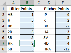
We can name this point value as “H_PTS_HR”.
If we’re later trying to determine how many points Javier Baez will earn from home runs, we can multiply Baez’s projected home runs by “H_PTS_HR” instead of multiplying by 9 or by cell B7 (in the image above).

If you’re familiar with the basic concepts of computer programming, setting the point value of home runs equal to a name is like using a variable.
The benefit of this is that we can later change the 9 to a different value. This is especially useful if we play in multiple leagues or if the scoring format changes.
It becomes very easy to change the scoring system without having to search within complex formulas. And we also don’t need to flip back and forth and remember that the HR point value was in B7 (as opposed to B6 or B8).
Using a name also gives the formula “meaning”. It’s a lot easier to understand this:
= B2 * H_PTS_HR
than it is to understand this:
= B2 * B7
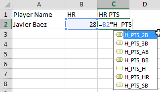
Another helpful benefit is that Excel makes all of your Names available through a type-ahead feature. So if you know you have a series of Names that start with “H_PTS_”, you can see all of them by typing out part of the name. This works no matter what tab of the Excel file you are on, meaning you don’t have to flip back and forth to figure out the exact cell holding the point value.
Using Cell Shading To Indicate Meaning
As we continue to build a spreadsheet that will eventually be quite complex, it can be helpful to indicate which cells are “input” cells and which ones are “calculated” (formula) cells. An easy way to denote this is by using cell shading (or coloring).
An “input” cell would be facts or assumptions that will later be used in formulas for calculating projected points and player rankings. For example, the number of points for each home run hit or the number of teams in the league.
A “calculated” cell will obviously be some kind of formula we enter in Excel.
The color coding will help remind you what cells you can change in the future (inputs) and what cells you should leave alone (formulas, calculations).
You can use your own color scheme, but for the rest of the series I will shade cells blue if they are “input” cells and a light red if they are “calculated” cells.
Not to mention that color coding your spreadsheets also offers a nice intimidation factor to your opponents at the draft table. Who knows, someone might just think twice about getting in a bidding war with you if you’ve got a kick ass spreadsheet on-screen.
Adjust For Your League’s Scoring Settings
The example league I’m using to create these rankings for is loosely based on a scoring system suggested for Fangraphs Ottoneu leagues. It is likely very different than the scoring system in your league. Accordingly, you will need to use judgment and tailor the steps below to fit your league’s specific scoring system.
STEP-BY-STEP INSTRUCTIONS
| Step | Description |
|---|---|
| 1. | Add a new sheet to your Excel file.A keyboard shortcut to add a new sheet is SHIFT + F11 at the same time.  |
| 2. | Right-click on the blank sheet and choose the option to “Rename”. 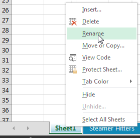 Name this sheet “Scoring Settings”. Name this sheet “Scoring Settings”. |
| 3. | Visit your league’s settings page and locate the list of point values for each stat category. On your “Scoring Settings” sheet, create a list of the various scoring categories and the point value for each. On your “Scoring Settings” sheet, create a list of the various scoring categories and the point value for each.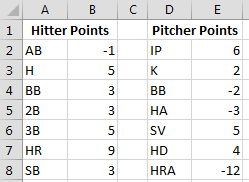 |
| 4. | In order to apply the concept of shading cells discussed above, I first place a border around the cells to point value cells.In my example file, I want to format cell B2. To do this click once on cell B2 and select the “Borders” drop down menu on the Ribbon. Then choose the “Outside Borders” option.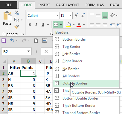 |
| 5. | Cell B2 will be an input cell that should be shaded blue. So while you still have B2 selected, click the “Fill Color” drop down arrow (the paint can icon) and click on the desired shade.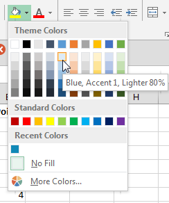 |
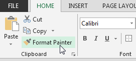
| 6. | To quickly format the other input cells, while still selected on cell B2, double-click the “Format Painter” icon (looks like a paint brush).Format Painter allows you to copy all formatting from one cell to the next selected cell. If you double-click on it, you can continue to click on many cells and they will all take on the formatting (a lot of people who know about Format Painter don’t know about the double-click option!).
We’re going to use Format Painter to make all the other point values blue and outlined. |
| 7. | In order to calculate projected points for all players, we will need to reference and use these scoring values in future formulas.To make it easier to reuse these figures, we will set them up as Named Cells. To do this, first click on one of your hitter point values (I’ll use B2 from my example).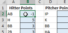 Then click on the “Formulas” tab of the ribbon and select the “Define Name” button. Then click on the “Formulas” tab of the ribbon and select the “Define Name” button. |
| 8. | In the window that pops up, enter a meaningful name that you’ll later be able to recognize. For example, to name the point value for At Bats, I chose the name “H_PTS_AB”.This will indicate this is the point value for hitter at bats.Click OK to save this name.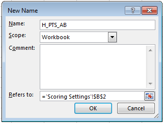 |
| 9. | Repeat this process for all of your hitting and pitching point values.I used these names for my hitting categories:
I used these names for my pitching categories:
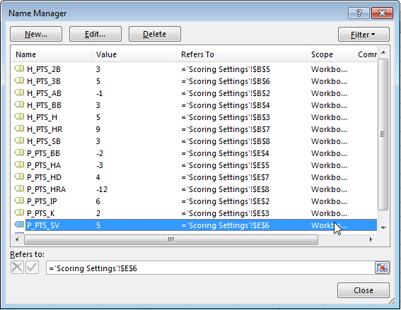
Note that Excel will not allow you to start a Name with a number (so you couldn’t name your cell “2B_PTS_H”). It may be a good idea to view the list of all names in your Excel file when you’re done. To do this, click on the “Name Manager” button of the “Formulas” tab. |
| 10. | We’re done. Save the file. |
Wrap Up
At this point in the process we have a file with projections, player IDs, and our league scoring settings. In the next part of this series we’ll start pulling the projection information into new sheets where we can begin to calculate each player’s projected points for the season. You can check out part three here or see all parts of the series in one place here.
Do You Have Any Questions?
If you have questions, it would be great if you can ask them in the comments below so others can benefit from the discussion.
If you’d like to know when I put out the next post in the series or similar posts in the future, click below to follow me on Twitter.

 While the Format Painter is still active (you can tell it’s active when you see the paint brush icon next to your cursor), simply click in all the other cells containing scoring point values.
 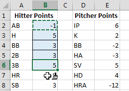 After you have selected all the point value cells, hit your ESC key to exit the Format Painter.
 Look over your list of names and make sure you haven’t missed anything.


Do you have any questions about Part 2? Please leave them here and I’ll do my best to answer them.
Hi there – I’m working through this tutorial for my weekly head-to-head league. We use R, RBI, SB, OBP and SLG for offensive categories. Should I simply be using a point value of 1 for each category?
Hi Jake, it sounds like you’re not in a points league and are in what I’d call a H2H “category” league. Unfortunately I don’t have anything written yet that specifically addresses those types of leagues. You could conceivably measure weekly standings for the league and get creative applying SGP, but I think there would be other methods like z Scores or percentage valuation methods that would apply better to H2H category leagues. I hope to tackle those methods one day, but have not gotten there yet.