So you’ve got a great set of projections, rankings, and dollar values.
This is great for draft preparation. But how do you take this information and use it during the draft? Is there a way to monitor the progress of the draft and see if you’re lacking in power compared to the others in the league? Do you need speed? Are you lacking in strikeouts?
You don’t need to buy draft software or a special draft spreadsheet. You can easily add a few more things to your Excel files and have a very powerful draft tool that can help you make these assessments.
I wrote about how to track drafted players in a spreadsheet last January. If you haven’t read that yet, please do. The instructions that follow pick up where that post leaves off.
Here’s how to calculate projected standings during your draft.
Prerequisites
I’ll be using Excel 2013 to create the projected standings. I think you’ll be able to follow a very similar process in Excel 2010 and Excel 2007.
 As I mentioned, this post assumes you have already added the named range and data validation drop down listing to select the team that has drafted a player.
This is how you will be tracking the draft selections during your draft. As each player is taken, you’ll locate them on your rankings/projections lists and select the team that drafted them.
I realize it’s a little early to be thinking about draft spreadsheets, but it’s top of mind for me now because I am participating in a mock draft that was coordinated by Bryan Curley of BaseballProf.com. I wanted to see how the draft is going and how teams stack up after the first few rounds. Not to mention you can set this up in your spreadsheet now and have it read to roll when we finally get closer to the season.
You can see the list of those participating in the mock draft in image above. As selections are being made in the draft, I’m marking them off in drop down I created in the “TAKEN” column.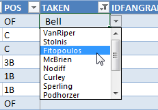
You may want to make several “fake” selections in your Excel file, just to have some data to work with. You will want to test that your projected standings are working prior to the draft… That’s the last thing you need to be monkeying on draft night.
Excel Functions and Features We’ll Be Using
There are a variety of ways to do this, but I’ll show you how to use a pivot table in this example. If you’ve never created a pivot table before, don’t worry. They’re a lot easier to work with than most think.
The pivot table will help us to quickly accumulate every team’s offensive stats (R, RBI, HR, SB, BA). Once we have the statistics accumulated in one nice table, we’ll then use the RANK formula to calculate the standings.
Pivot Tables
Pivot tables are very useful for taking a lot of lines of data (like we have on our “Hitter Ranks” tab) and combining or summarizing that data into more easily or digestible parts.
For example, your listing of all hitters and their projections is probably hundreds of rows of information. If you were to select 14 hitters for each of the 12-teams in your league, that would be 168 hitters. Sorting all of those players into teams and then calculating the totals for five different categories for each team might seem like a daunting task.
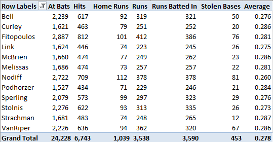
The good news is that creating a pivot table can be done in only a few clicks of the mouse and within minutes you can have a table that looks just like this:
Rank (or RANK.EQ) Formula
These two formulas are essentially the same; however, RANK was discontinued in Excel 2010 and was replaced by RANK.EQ.
If you’re using Excel 2010 or later, either one should work. But if you are using Excel 2007 or earlier, you must use RANK (RANK.EQ didn’t exist then).
These formulas will interpret a list of numbers and return the ranking of a specified item in the list. We can use this to analyze the entire list of player SGPs and give us a ranking for each player (e.g. Mike Trout is #1).
The formulas require three inputs:
RANK(Number, Ref, Order)
RANK.EQ(Number, Ref, Order)
- Number – This is the specific number you want ranked. If your goal is to figure out where your team ranks in total home runs, you would select the individual cell containing your team’s projected home runs.
- Ref – This is the range of data, or the list of data, to calculate the ranking from. Continuing with the total home runs example, you would select the entire listing (or range) of projected home runs for all teams in the league.
- Order – Technically this is not a required part of the formula, but using it can make our lives a little easier. If you leave this part out of the formula, Excel would return a “1” for the team with the most home runs and a “12” for the team with the least home runs. You can see we don’t really want to know our “Rank”. We’re looking for “Rotisserie Points”. We would like the top team in home runs to show a “12”. The “Order” parameter in the RANK function is looking for a zero or a one. If you leave it blank or put in a zero, the RANK function gives a “descending” ranking. This is the typical ranking where “#1” is the best or highest possible ranking. We are looking for an “ascending” ranking, where a “12” is the best result. To do this, just put a one in for this piece of the function.
Step-by-Step Instructions
Don’t be intimidated by the number of steps here. You should be able to perform them pretty quickly.
| Step |
Procedures |
| 1. |
To guard against theoff chance that something goes wrong, create a backup copy of your projections/rankings spreadsheet.Do this by performing a “Save As…” or copying your existing file and putting another copy somewhere for safe keeping. |
| 2. |
Click on a piece of data on your “Hitter Ranks” tab, where you have the projected stats for each player and where you are tracking the drafted players.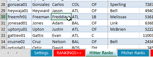 Then click on the “Insert” tab. Finally, click on the “Pivot Table” button. Then click on the “Insert” tab. Finally, click on the “Pivot Table” button.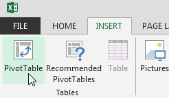 |
| 3. |
The “Create PivotTable” menu will pop up. If you’ve set your rankings up in a table (another reason I love using tables!), Excel should recognize this and select the whole table for the “Table/Range:” input.
If Excel isn’t recognizing your data, click the button on the “Table/Range:” input and select your data using your mouse.
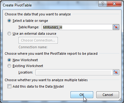
Choose the option to create the PivotTable on a “New Worksheet”.
Click “OK”.
|
| 4. |
You should now see the placeholder for a PivotTable.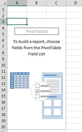
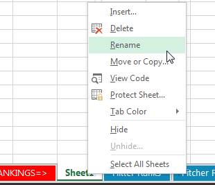
Right-click on the newly created sheet and choose to “Rename” it. Call this new tab “Projected Standings”.
|
| 5. |
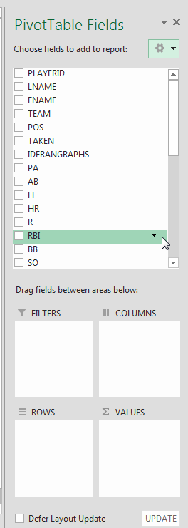 Toward the right of your screen, you should see the list of all fields in your data. Toward the right of your screen, you should see the list of all fields in your data.
Then toward the bottom right of the screen you’ll see four areas labelled “FILTERS”, “COLUMNS”, “ROWS”, and “VALUES”.
Setting up a Pivot Table is as easy as dragging fields into one of those four areas. It’s simply clicking and dragging to build a table to fit what you want to see.
|
| 6. |
At this point, it’s helpful to have a vision of what you’re trying to produce. We all know what the rotisserie standings look like:

Now it’s simply an exercise of clicking and dragging items. We want our “ROWS” to be the team drafting the player. That information is stored in the “Taken” column of my example file.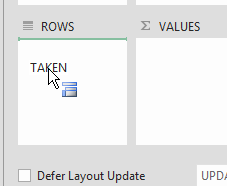
To accomplish this, click and drag the “TAKEN” field from the “PivotTable Fields” section and drop it onto the “ROWS” area.
|
| 7. |
If you have populated any “fake data” in the “Taken” column, you will see those names populate into the Pivot Table.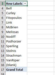 |
| 8. |
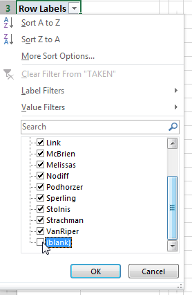 Notice how the listing of teams also has a “(blank)” item? This would represent any player with nothing in the “Taken” column. Or undrafted players. Notice how the listing of teams also has a “(blank)” item? This would represent any player with nothing in the “Taken” column. Or undrafted players.
We don’t want that messing up our standings data, so we need to filter it out.
Click on the drop down arrow in the cell that says “Row Labels”. This will show you the filtering menu you may be familiar with on the other tables we’ve worked with in the past.
Scroll down to the end of the listing and uncheck the “(blank)” item.
Click “OK”
|
| 9. |
Think again about what our projected standings will look like. We want the sum of all AB, H, HR, R, RBI, SB, and a calculation of Batting Average to appear. To get the sum of these statistics, we want to drag them from the listing of all fields and drop them onto the “VALUES” area. To get the sum of these statistics, we want to drag them from the listing of all fields and drop them onto the “VALUES” area.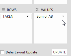 When you drop them, you should see Excel label them as “Sum of [category]” (for example, “Sum of AB”). If you see “Count of [category]”, be patient. We’ll fix that shortly. When you drop them, you should see Excel label them as “Sum of [category]” (for example, “Sum of AB”). If you see “Count of [category]”, be patient. We’ll fix that shortly.
Click the drop down arrow on the “Sum of [category]” label and choose the “Value Field Settings…”
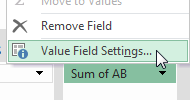 This screen is where you can customize the description of the column (“Sum of AB” is not a sexy column name) and change from “Count of” to “Sum of”, if necessary. This screen is where you can customize the description of the column (“Sum of AB” is not a sexy column name) and change from “Count of” to “Sum of”, if necessary.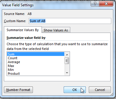 Note that you cannot name the column “AB” because that’s the name of a field in the table. That’s why I labelled mine “At Bats”. Sure beats “Sum of AB”… Note that you cannot name the column “AB” because that’s the name of a field in the table. That’s why I labelled mine “At Bats”. Sure beats “Sum of AB”… |
| 10. |
Repeat step 9 in order to add H, HR, R, RBI, and SB.
Then let’s clean up the formatting. Use your mouse to select all the numbers in the table.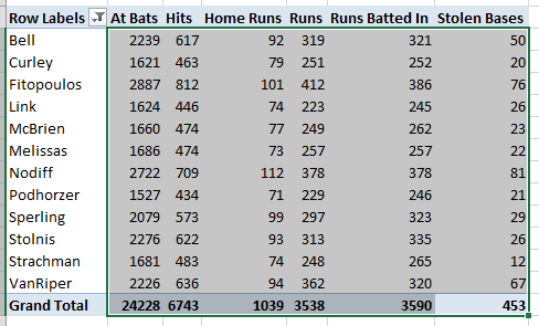  Then click the “Comma” number style and decrease the decimals two times (to remove the decimals). Then click the “Comma” number style and decrease the decimals two times (to remove the decimals). |
| 11. |
The last piece of information we need is batting average, which you probably realize is a calculation of the “At Bats” and “Hits” columns we just added.To add a calculated field, first select any cell within your Pivot Table. Then notice the “PIVOTTABLE TOOLS” menu that appears on the Excel ribbon.
If you’re in Excel 2013, click on the “ANALYZE” tab (I believe it’s “OPTIONS” in Excel 2010). Then click the “Fields, Items, & Sets” drop down. Finally, click the “Calculated Field…” option.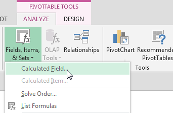 |
| 12. |
Once the “Insert Calculated Field” dialog pops up, replace the “Name:” field with “Average”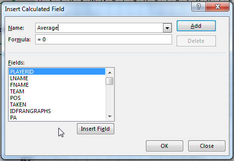 In the “Formula:” field, replace the “=0” with our calculation of batting average, “=H/AB”. Instead of typing the formula, I recommend double-clicking on the field names for “H” and “AB” (you can type the “=” and “/”). In the “Formula:” field, replace the “=0” with our calculation of batting average, “=H/AB”. Instead of typing the formula, I recommend double-clicking on the field names for “H” and “AB” (you can type the “=” and “/”).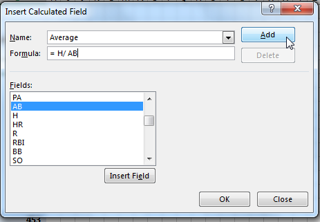 Make sure to click “Add” when you’ve given the name and formula calculation. Make sure to click “Add” when you’ve given the name and formula calculation. |
| 13. |
Excel added this as a “Sum of Average” column for me. So again, I need to go into the “Value Field Settings…” for this and rename it to “Batting Average”.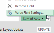 Then select the values in this column and increase the decimals three spots so it looks like an actual batting average. Then select the values in this column and increase the decimals three spots so it looks like an actual batting average.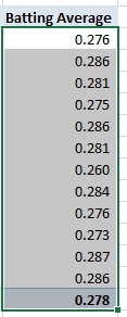 |
| 14. |
We’ve created our vision! But you’re probably thinking, “That’s a projected statistics table, but it isn’t showing me the projected standings…”We will now add a second block of formulas below this table to convert the statistics into “standings”.
But first, we need to adjust a setting on the Pivot Table we just created. Use your mouse to select any cell in the Pivot Table and then click on the “PIVOTTABLE TOOLS>ANALYZE” tab (or PIVOTTABLE TOOLS>OPTIONS” in Excel 2010). Once on this tab, click on the “Options” drop down menu all the way to the left of the ribbon (underneath the “PivotTable Name” area). Make sure the “Generate GetPivotData” option is UNCHECKED. Once on this tab, click on the “Options” drop down menu all the way to the left of the ribbon (underneath the “PivotTable Name” area). Make sure the “Generate GetPivotData” option is UNCHECKED.
There may be ways to get this to work with it checked, but I find it confusing and don’t like the way things work when this is checked.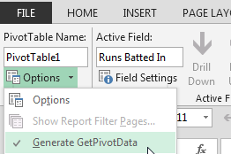 |
| 15. |
Copy the headers from the Pivot Table for “Home Runs”, “Runs”, “Runs Batted In”, “Stolen Bases”, and “Average”. Paste the headers below the Pivot Table. Leave a column to the left of the headers (I pasted them in column B, leaving column A open). Paste the headers below the Pivot Table. Leave a column to the left of the headers (I pasted them in column B, leaving column A open).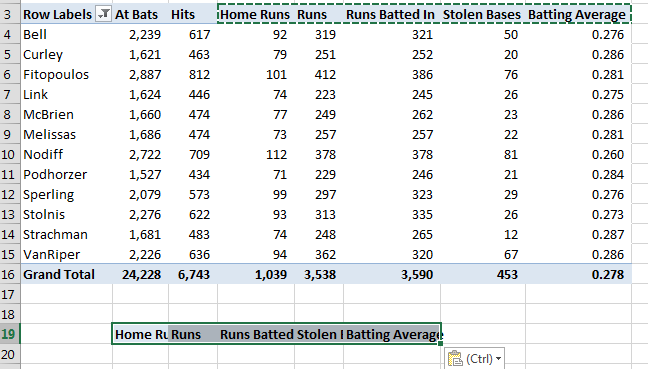 |
| 16. |
Now copy the team names from the Pivot Table (skip the “Row Labels” and the “Grand Total” items). Paste the team names along the side of the headers pasted in the last step.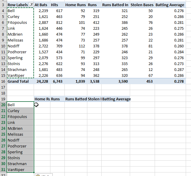 |
| 17. |
 Your Pivot Table may be positioned slightly different than mine. I’m now going to add a formula to cell B20 (in the image above). Add your formula so that it will calculate the “Home Runs” for the first team. Your Pivot Table may be positioned slightly different than mine. I’m now going to add a formula to cell B20 (in the image above). Add your formula so that it will calculate the “Home Runs” for the first team.
After you’ve selected the cell, click the “Insert Function” button on the Excel toolbar.
Search for the “RANK” formula. Select it from the list and hit “OK”.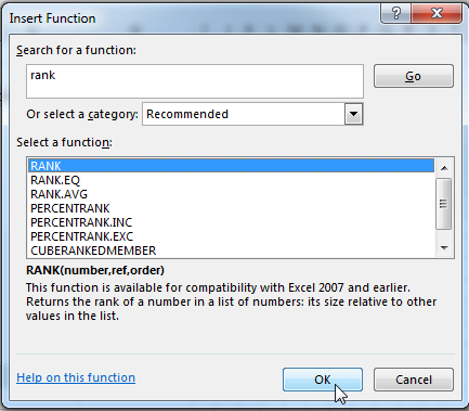 |
| 18. |
Again, your Pivot Table may not be located exactly where mine is. Here’s my exact location so you can translate the formulas to the location of your Pivot Table.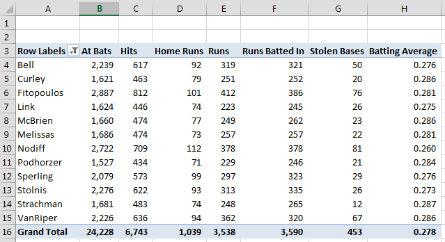 And here are the inputs into the formula. And here are the inputs into the formula.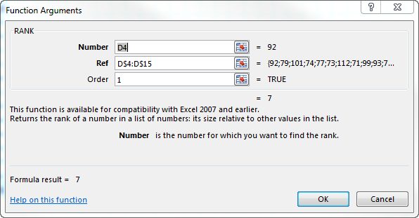 Recall from the explanation of the RANK formula, at the beginning of the post, that the “Number” argument is the specific item you want a ranking for. In this case, I want to rank the number of home runs for my team (“Bell”). My homers are listed in cell D4, so that becomes my entry into the “Number” field. Recall from the explanation of the RANK formula, at the beginning of the post, that the “Number” argument is the specific item you want a ranking for. In this case, I want to rank the number of home runs for my team (“Bell”). My homers are listed in cell D4, so that becomes my entry into the “Number” field.
The “Ref” argument is the range or grouping of every team’s home runs. That range is from cell D4 to cell D15. We will eventually be dragging this formula to all the other teams and columns in the projected standings are we are creating. We know that the “range” for each category will always be in cell rows 4 through 15. We don’t want that range to move as the formula is copied, so we use the “$” to convert this to an absolute cell range (D$4:D$15).
Finally, we want our ranking to be given in descending order so that the team with the most home runs gets a “12” instead of a “1”. To accomplish this, we put a “1” in the “Order” field.
Click “OK” to accept this formula. My completed formula (yours may differ slightly if you created your tables in different spots) is:
=RANK(D4,D$4:D$15,1)
NOTE: The “1” at the end of the formula is necessary for categories where higher totals or a higher average are better. Most offensive categories fall under this category. However, when calculating rankings for pitching ratios, like ERA and WHIP, where a lower average is better, change the “1” to a “0”.
|
| 19. |
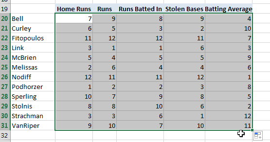
After the formula is completed, click once to select the cell containing your formula. Then hover your mouse over the black box in the lower right corner of the cell. You should see the cursor change to a plus sign.
Click the black box and drag it so that the formula copies to all teams in your list (TIP: double-clicking on the black box will also copy it down to the end of the column and you won’t need to click and drag).
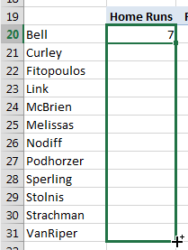
Look over your rankings to make sure they seem appropriate.
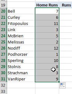
Then click the black box again and now drag it to the right, in order to copy the rankings formulas to each stat category.
|
| 20. |
The final step is to calculate the total points for each team. Create a “Total” column header next to the “Batting Average” column.
Below this column header, use the “SUM” formula to add across for each team. In my specific example, the formula for the first team is:
=SUM(B20:F20)

|
| 21. |
Copy this formula down (using the black box). You’ve now got projected standings (for hitters at least).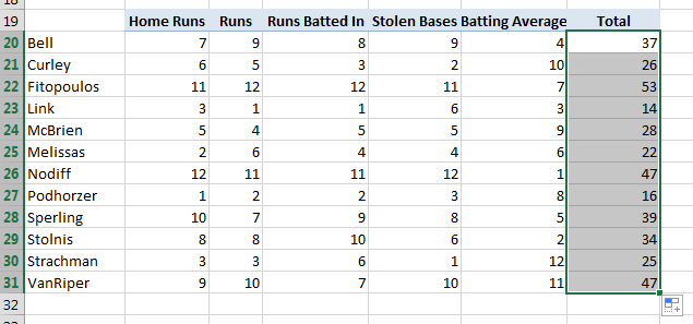 |
| 22. |
The last thing to keep in mind is that Pivot Tables do not automatically update like most other Excel formulas. If you continue to mark additional players as drafted, you won’t see the updated standings immediately.
To update a Pivot Table, right-click on any cell inside the table and click the “Refresh” button.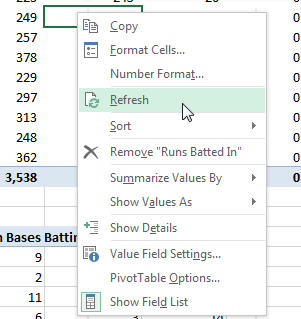
|
Wrapping Things Up
If this is your first foray with Pivot Tables, hopefully you’ve realized “they’re not that bad”. They intimidated me for a long time, but once you get the hang of it, it’s very easy to find interesting information.
They could be used to calculate the effect of a trade in the middle of the season. Or to simply view the combined effect of a multi-player deal. If you’re evaluating a 4-for-4 trade, you could calculate the total statistics for each side very quickly.
The hardest part of this whole exercise wasn’t creating the Pivot Table! You can do that in a few mouse drags.
The Mock Draft
The steps above will work for any draft in any season, but if you’re interested in following the results of this early mock draft as you prepare for the 2015 season, you can see the live draft room here or see the team-by-team results here.
Thanks For Reading
If you’d like more tips and step-by-step instructions like this, please sign up as a Smart Fantasy Baseball Insider in the registration box below. I won’t flood your inbox. I send about one e-mail each month. It might include a rankings spreadsheet, a how-to article, and a summary of what’s new at the site since the last newsletter.
Or if e-mail’s not your thing, please follow me on Twitter to get notified of new postings.
 As I mentioned, this post assumes you have already added the named range and data validation drop down listing to select the team that has drafted a player.


 Then click on the “Insert” tab. Finally, click on the “Pivot Table” button.


 Toward the right of your screen, you should see the list of all fields in your data.

 Notice how the listing of teams also has a “(blank)” item? This would represent any player with nothing in the “Taken” column. Or undrafted players.
 When you drop them, you should see Excel label them as “Sum of [category]” (for example, “Sum of AB”). If you see “Count of [category]”, be patient. We’ll fix that shortly.
 This screen is where you can customize the description of the column (“Sum of AB” is not a sexy column name) and change from “Count of” to “Sum of”, if necessary.
 Note that you cannot name the column “AB” because that’s the name of a field in the table. That’s why I labelled mine “At Bats”. Sure beats “Sum of AB”…
 Then click the “Comma” number style and decrease the decimals two times (to remove the decimals).

 In the “Formula:” field, replace the “=0” with our calculation of batting average, “=H/AB”. Instead of typing the formula, I recommend double-clicking on the field names for “H” and “AB” (you can type the “=” and “/”).
 Make sure to click “Add” when you’ve given the name and formula calculation.
 Then select the values in this column and increase the decimals three spots so it looks like an actual batting average.
 Once on this tab, click on the “Options” drop down menu all the way to the left of the ribbon (underneath the “PivotTable Name” area). Make sure the “Generate GetPivotData” option is


 Your Pivot Table may be positioned slightly different than mine. I’m now going to add a formula to cell B20 (in the image above). Add your formula so that it will calculate the “Home Runs” for the first team.
 Recall from the explanation of the RANK formula, at the beginning of the post, that the “Number” argument is the specific item you want a ranking for. In this case, I want to rank the number of home runs for my team (“Bell”). My homers are listed in cell D4, so that becomes my entry into the “Number” field.


This is amazing. Really cool.
Thanks, Simon!
Hey Tanner – any thoughts on how to tweak this for leagues that have benches (deep ones at that)? I believe that this method will simply calculate a running total of stats for all players drafted by a team. Obviously that works great for a league with no benches, because all the stats are for starters, but in a league with benches I want to calculated projected standings based on the starters only. I’d imagine I’d have to keep track of everyone’s rosters and determine if the player is a starter or bench player for that team, and then calculate standings for only starters’ stats.
Hi Will,
When you set up the drop down menu to list out teams in your league, I think you’d have to set up a “bench” team for each. For example, “Team A – Bench”, “Team B – Bench”. Then as bench players get drafted, you would put them on the bench team and not the “regular” team.
You could then filter the bench teams out of the pivot table (there’s a way to add a filter to a pivot table so not all items are pulled into it) OR you could just not include the bench teams in the ranking formulas you create.
Hope that helps.
Tanner
Hi Tanner, Just wondering if you could walk thru the pitching side? I am having issues with ratios. Tnx!
Hey Ben, that’s a good idea. I should tackle that sometime soon. But in the meantime, if I had to guess about the biggest challenge in doing this for pitching, it would be the fact that the ratios are in inverse rank order, meaning the lowest ERA and WHIP get the most rotisserie points.
You can do this pretty easily by changing the last argument in the RANK formula.
Using the example above, if you wanted to flip the point value for this formula: =RANK(D4,D$4:D$15,1)
You would simply change the last “1” to a “0”, or =RANK(D4,D$4:D$15,1)
The other challenge may simply be calculating the ratios. Similar to how AB and H were pulled, in the example above, to calculate AVG, you’d need to pull the totals for IP, H, BB, and ER to calculate WHIP and ERA.
Let me know if this doesn’t help you and you have a more specific question after trying these things out.
OK, thanks Tanner. I get the idea now, just wasn’t sure about the formula. Thanks again!
I am looking to track projected standings in the middle if the season. Any tips for capturing actual stats and then adding remainder of year projections to determine this? Tough factors: injuries, trades, projection adjustments, and how much a team uses its bench. Thanks.
Hi Mike,
I do need to get around to writing this. It’s not something I’ve fully tackled yet. I can try to speak at a very high level about what I’d do.
1. Hopefully you have a league provider that allows the “public” to see your league standings. Not all of them do this. ESPN, for example, doesn’t by default (I don’t think), but there is a setting where the commissioner can make your league visible to the public. This is helpful because you could then use Excel or Google Sheets to import your live standings data.
2. You’d need to regularly download and import (copy & paste) in “Rest of Season” (ROS) projections. Fangraphs provides several different ROS projections .
3. Once you have this data in a file, you could then use formulas to add each teams projected player stats to the stats they have already accumulated.
Like you mention, bench players are an interesting wrinkle in this. I think you’ll have to manually maintain who each teams starters are in your file. Or if your league is public, you may be able to download each team’s roster. But that’d be a lot of work to set up.
This isn’t elegant. But a perfect solution would be very hard to fully automate.
Thanks,
Tanner