In my last post about how to calculate positional rankings in your player spreadsheet (link), I realized a weakness in the approach I outlined. I’m here to fix that with a slightly more complex formula. 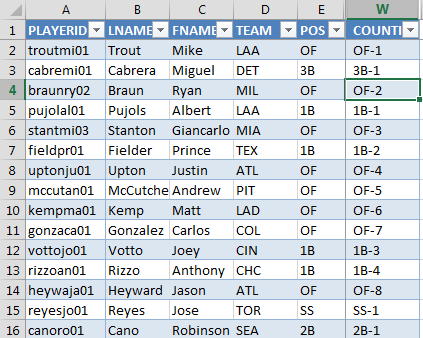
The Weakness In The First Approach
The problem with the first approach is that it is entirely dependent upon how the file is sorted. If the file is sorted by dollar value or standings gain points in descending order, then the rankings work.
But if you sort the file by home runs, stolen bases, or player name, then the rankings fall apart. The player with the most home runs (or the most stolen bases or the first name alphabetically) becomes the top ranked player.
The COUNTIFS Excel Function
Instead of the COUNTIF function, we’ll use the COUNTIFS function this time.
You might remember from the last post that the COUNTIF function will count the number of cells in a specific range that meet a specified condition (e.g. “Hey Excel, count all the players in this column that have a ‘POS’ of ‘OF’.”).
Well the COUNTIFS function counts the number of cells in a specific range that meet all of the conditions you provide (you can give multiple conditions).
In plain English, our goal is to have Excel count all the players in our list of hitters that have a “POS” of “OF” AND that have a higher projected SGP than our player being evaluated.
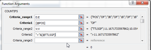
We’ll get into the specifics of our formula in a bit, but here’s a screenshot of the Excel formula wizard for our COUNTIFS function.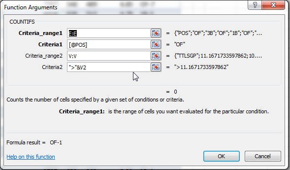
This formula allows for an open-ended number of arguments, but you do need to pieces of information for each set of criteria you want to specify. Each criteria requires:
- Range – This is the block, column, or area of cells we want to count from. “Excel, look in Column E and count the cells that meet this condition I’m about to tell you about in bullet #2.”
- Criteria – This is what we are evaluating the cells for. “Count the cells in Column E that show ’1B’ as the position.”
If we want to specify three conditions that must be met, then we would need six arguments (three ranges and three criteria: range1, criteria1, range2, criteria2, range3, criteria3).
Step By Step Instructions
| Step | Description |
|---|---|
|
1. |
I’m going to build this formula in pieces. First, create a new column to hold “COUNTIFS RANK”. To do this, just type the column header to the right of your existing table information. We’ll start with just the COUNTIFS formula for now. |
|
2. |
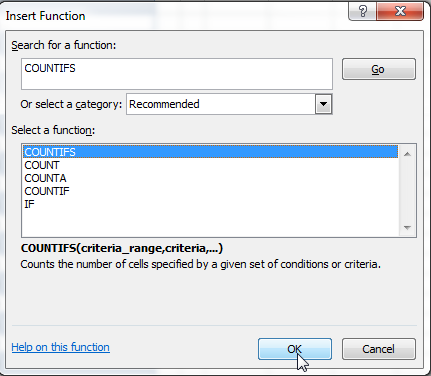
I’ve hidden a lot of information in my rankings. For now, we’ll just need the “POS” column and the “TTLSGP” column (or whatever measure you’re using to evaluate players, like maybe total points or projected dollar value). Click in the first empty cell of your “COUNTIFS RANK” column (cell W2 in my example). Then click on Excel’s “Insert Function” button (fx icon next to the formula editor). Search for the COUNTIFS function and hit “Go”.
|
|
3. |
After you’ve located COUNTIFS, hit “OK”. The first range we’ll be evaluating is the “POS” column. In my example file, “POS” is in column E. To have Excel look through all of column E we can enter “E:E” in the “Criteria_range1” field. |
|
4. |
Mike Trout happens to be atop the spreadsheet right now. In order to count only players with the same position as Trout, we’ll click in cell E2 (where Trout’s position is located). Excel will convert this to it’s Structured Reference notation which is [@POS]. |
|
5. |
The second range we’ll be evaluating is the “TTLSGP” column (or whatever you’re ranking players by).In my example file, “TTLSGP” is in column V.My intention is to have Excel look through all of column V and count players that have higher “TTLSGP” than each given player. To have Excel look through all of column V we can enter “V:V” in the “Criteria_range2” field. |
|
6. |
Remember, we’re currently building the formula in Mike Trout’s row and we’re trying to find players with greater SGP than him. We’re essentially trying to put “>[@TTSGP]” (or “>V2”) in this box for “Criteria2”. The problem is we want Excel to treat the “>” as text but the “[@TTLSGP]” as a structured reference/cell number. To specify text in Excel you surround it with double quotes. And you will hopefully recall from the first positional rankings piece that we can build text strings using the ampersand. So to create this, we want to enter “>”&[@TTLSGP] into the Criteria2 cell. Or you could use the traditional cell number convention. |
|
7. |
You’ll know this is working when you see “>11.167” off to the right (this is a preview of what Excel is thinking). We want Excel to look for any player with standings gain points greater than 11.167.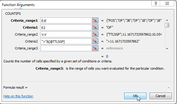 |
|
8. |
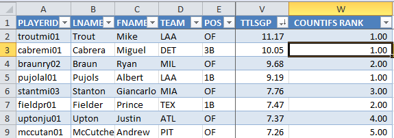
After you accept the formula you’ll see that we need to tweak it some. It’s counting players that have greater TTLSGP. Nobody has a greater SGP than Trout so it’s evaluating to zero. We want to add a 1 to the result of our COUNTIFS formula. This will reflect rank instead of count how many players are better. Edit the existing formula by putting “+1” at the end. =COUNTIFS(E:E,[@POS],V:V,”>”&[@TTLSGP])+1 You can see this fixes our issue by making Trout #1, Braun #2, etc. |
|
9. |
In the next step we’ll add in the text part of each player’s position (to make Trout “OF-1”). Before we do that, wrap our existing formula in parentheses so it doesn’t interfere with the “OF-” part we’ll soon be adding. =(COUNTIFS(E:E,[@POS],V:V,”>”&[@TTLSGP])+1) |
|
10. |
Now we can add in the text part of the positional rankings. Click your mouse so that it’s between the equals sign and the opening parenthese we added above. We’re trying to add the position in front of the number rank. Click on the “POS” column for the row you are editing the formula for. Then type the following: &”-“& This will append the player’s position to the ranking we calculated earlier and put a dash in between. My final formula is: =[@POS]&”-“&(COUNTIFS(E:E,[@POS],V:V,”>”&[@TTLSGP])+1) |
|
11. |
Hit Enter. We’re done!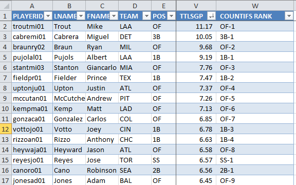 |
That’s Better
I apologize for sending you down the wrong road with the last post. This formula is clearly better.
This ranking does not depend on how the file is sorted. Excel is calculating each players ranks explicitly according to the TTLSGP column.
You might notice it takes a while for your Excel file to calculate now. The formula we added takes much more resources because it’s comparing every player to every other player in the whole spreadsheet.
Have Other Questions About How To Do Things Like This?
I’m serious. Ask me!
If you have questions about how to make an awesome rankings or draft spreadsheet, let me know. You can comment below or e-mail me at smartfantasybaseball at gmail dot com.
If you’re interested in similar articles in the future, following the site on Twitter or registering as an Insider are the best ways to keep up-to-date.




 If you don’t like the Structured Reference notation, you can manually type in “E2” and get the same result.

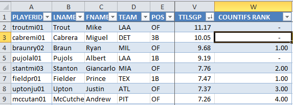 We actual want Trout’s rank, not how many are higher than him. His rank is first. The second player, Ryan Braun, is evaluating to a 1. But really he’s the second ranked outfielder.


Any luck with making it pick up 1B and OF separately for a guy that is dual-eligible? Thanks!!
Yes. Just went live now. https://www.smartfantasybaseball.com/2014/09/how-do-you-account-for-and-value-players-with-multiple-position-eligibility/
Sorry for the delay. As I started to write that one to answer your question, I realized that this one had to come first.
Hope it’s what you are looking for. It’s tough to accommodate it well in a spreadsheet.