How To Track Drafted Players In A Spreadsheet

I’ll paraphrase a reader question I recently received:

Hey, you with your big fancy spreadsheets.  I need a way to easily hide the players that have already been drafted so I don’t waste time digging around in a bunch of players that are no longer available.  Have any tips?

– Bill

Great question.  Let me show you how I do this.

But First…

We have three key Excel concepts or features you should understand.  If you’re already familiar with these, just skip down to the step-by-step instructions below.

1. Named Ranges
2. Data Validation
3. Filtering

Named Ranges

Excel allows you to create names for groups or blocks of cells.  Once established you can use this name in formulas instead of having to fully spell out the entire range of data again.  I find it a lot easier to deal with a name like “TeamNames” than it is to explicitly specify the area of a range like “Settings!$A$1:$A$10”.  Named ranges are a lot easier to remember and a lot less likely to result in errors.

Data Validation

Data validation ensures that information entered in a cell or calculated by the Excel fits specified criteria.    You could validate that information entered in the cell is a date or is larger than 0, for example.

In the example below we will create a drop down menu that lists each team in your fantasy league and validates that the selected value is spelled correctly and corresponds to a team in your league.

Filtering

Filtering is a function in Excel that allows you to hide entire rows of data that don’t meet certain requirements.  In this example we will filter the list of players to hide players that have been given a team (they have been drafted).

Step-By-Step Instructions

The following instructions will take you through the process of adding a column to track which players have been drafted and which team in your league selected each player.  We will create a drop down menu that lists all teams in your league and use this to document who was drafted and by what team.

These instructions assume you have some kind of a starting spreadsheet containing projections and rankings already.  If you don’t have such a starting point, skip to the end of this post for information on how to get here.

Step	Procedures
1.	Locate a large blank area somewhere in your spreadsheet where you can list out all your teams.  One way to do this is to create a new tab called “Settings”.
2.	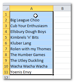Create a list of all the teams in your league within the blank area you identified.Leave the first cell in the list blank.  Then list out the teams in your league in alphabetical order.  After you have listed all the teams in the league, use your mouse to select the blank cell and all the teams (click-and-drag to select).
3.	Go to the “Formulas” tab of the Excel Ribbon and click the “Define Name” button.
4.	In the ensuing menu, enter “Teams” in the “Name:” field.  Leave everything else as is and click OK to accept the change.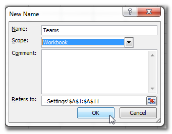
5.	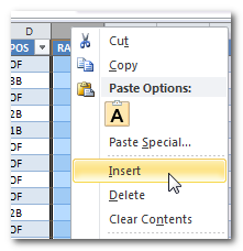Go to the rankings or projection tab in your spreadsheet where you want to track the draft progress (or to mark players as drafted).We must add a column to this tab. Recall that newly inserted columns insert to the left of a selected column.  So right-click on the column you want the new column added before and choose the “Insert” menu option.
6.	Give the column a header name (I chose “LGTEAM” for “League Team”).
7.	Click once in the first blank cell beneath this new column header (in my example above I would click in cell E2).After selecting this cell click on the “Data” tab and then the “Data Validation” button (either click on the top of the “Data Validation” button or if you click on the drop down piece then choose the “Data Validation…” menu option.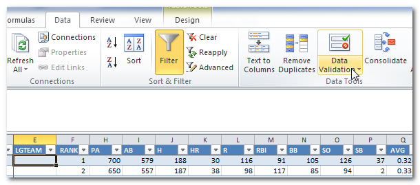
8.	In the ensuing menu, choose the “List” option in the “Allow:” drop down menu.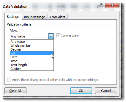
9.	In the “Source:” field, enter the formula “=Teams” (this is the name of the range created in step 4 above).  This tells Excel the list of names for our drop down comes from the “Teams” range created earlier.  Click OK to close this window.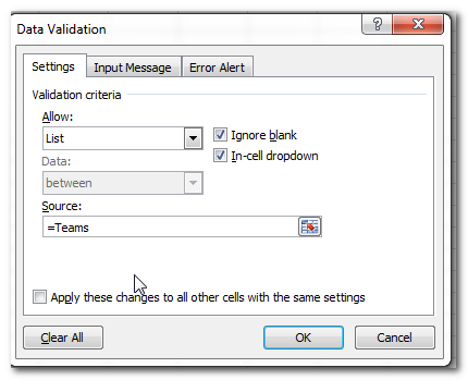
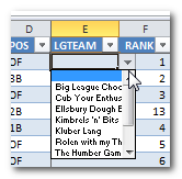
10.	Test that the drop down menu is working.  When you click on the first cell in the “LGTEAM” column, you should now see a drop down menu that lists all of your competitors.
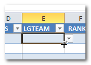
11.	We must now copy this drop down menu to all the cells in the column.  To do this to place your cursor over the lower right hand corner of the cell.  As your mouse reaches this corner the cursor should turn into a black cross or plus symbol.  When you see this, left-click your mouse and hold the button down while you also drag your mouse to the bottom of the entire column.Alternatively, you can select the cell with the drop down menu and copy the contents (CTRL+C).  Then select every cell beneath it and paste the contents (CTRL+V).Afterwards you should have the drop down menu on each cell.
12.	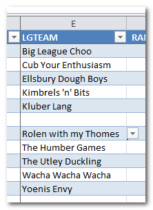As players begin to be selected during the draft, use the drop down menus to select the team they’ve been chosen by.  This will leave some blank cells and some cells with team names in them.
13.	Use Excel’s filtering capabilities to only display undrafted players.  To do this, first make sure you have clicked the “Filter” button on the “Data” tab.  This will add drop down menus to each column header.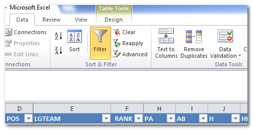
14.	Click the drop down menu atop the “LGTEAM” column.  You should see a menu appear with a check box for each team that has selected players so far.  Click the “(Select All)” check box.  This will remove all check boxes in the list.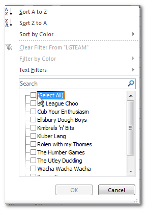Scroll further down the list and check the “(Blanks)” option.  Then click OK.
15.	All drafted players will disappear and you will only see players that are still available.As you continue to select teams for more players, those players will not automatically hide but you can quickly reapply the filter.  To refresh the list just click the filter drop down menu and then click “OK” (you don’t even need to monkey around with the team check boxes again).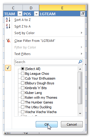

This Looks Awesome, But I Don’t Already Have A Rankings/Projections Spreadsheet

Don’t worry.  If you don’t already have your own spreadsheet, you can register as an SFBB Insider (it’s free) and get a free 60-page guide showing how to create your own Excel-based rankings.  Or if you want to get your hands dirty and create your own projections, check out the “SFBB ‘Projecting X’ Bundle” that comes with Mike Podhorzer’s book “Projecting X” (the best tutorial I’ve found for developing your own projections) and an Excel template for following the “Projecting X” method that comes preloaded with 800 players, links directly to Fangraphs pages for each player, and that will rank players for you automatically.

What Questions Can I Answer For You?

Have a question about how to do something in Excel?  Or how to use one of the spreadsheets discussed on the site?  Or do you just wonder if it’s possible to do something?  E-mail me at smartfantasybaseball@gmail.com with your question.

Thanks!

Be smart.