Create Your Own Fantasy Baseball Rankings: Part 4 – Pitcher Rankings

Welcome to the fourth part of the “Create Your Own Fantasy Baseball Rankings” series.  If you missed an earlier part, you can find it here.  You can start at almost any part of the series, but it’s not recommended you start with Part 4 unless you are very familiar with the Excel functions listed below.  Part 4 is essentially reperforming step 3(which focused on hitters) for pitchers.  This post assumes you are familiar with the Excel functions and formulas used in Part 3.

Please note that this six part series has been adapted into a 10 part book that also shows you how to convert standings gain points into dollar values and how to calculate in-draft inflation.

A few notes about the series:

• It was originally written before the 2013 MLB season.  The screenshots and player references you see might refer to things from that time frame, but the same approach will work today.
• If you register as SFBB Insider, you can receive all six parts in a free, tidy, and easy-to-use e-book
• Familiarity with Excel is recommended, but I do my best to explain all formulas and functions used
• Some of the formulas used in the series do not work in Excel for Mac computers.  I apologize for this.  I don’t understand why Excel isn’t built to operate the same on that platform.

In this fourth part of the series we will use Excel formulas and functions to start pulling pitcher information (name, position, team) and projection information in order to eventually calculate our own rankings.

EXCEL FUNCTIONS AND FORMULAS IN THIS POST

Below are the Excel functions and formulas used in this post.  If you would like more background on them, please refer to Part 3 or ask questions in the comments area below.

• VLOOKUP
• TABLES and NAMED RANGES
• COLUMN

STEP-BY-STEP INSTRUCTIONS

1. Staying consistent with the hitting projections, I’m going to use the free Steamer projections from Fangraphs.
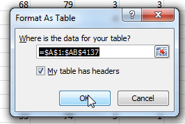
2. To make the pitching projections easier to work with, convert the “Steamer Pitchers” tab to a “table” in Excel.  To do this, click anywhere within the data on the “Steamer Pitchers” worksheet.  Then locate the “Home” tab in the Excel menu system (“the ribbon”).  Click once on the “Format as Table” drop down, and then select your desired color scheme.You will then be prompted to verify the range of cells in the table and that your table has a header row (e.g. Name, W, L, ERA, etc.).  Check “My table has headers”.  Click OK.
3. Because we’ll later be these pitcher projections into other worksheets, it will help us greatly if the fangraphs player ID is the first column of the table (you can use the VLOOKUP formula if the player ID is in the first column, otherwise you’re stuck using more difficult and/or multiple formulas).  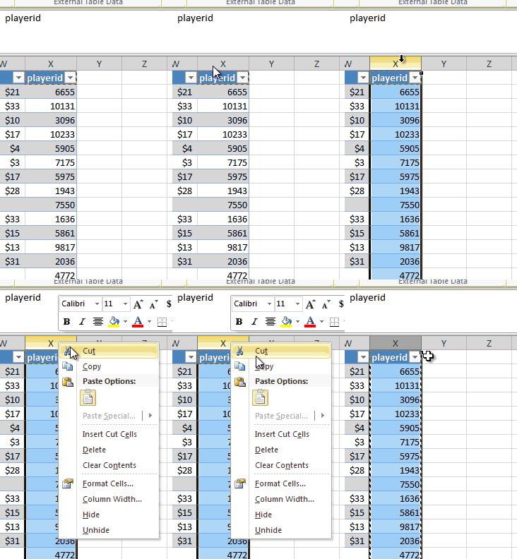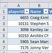Right-click on the top of the fangraphs player ID column (should be column X in the Steamer Pitchers projections).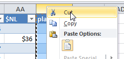Now right-click on the top of the player name column (column header “A”) and select “Insert Cut Cells”.  When you’re done, you should have the “playerid” column first and “Name” second.
4. Before we finalize this table, we must give it a name.  Go to the “Formulas” tab on the Excel ribbon and click on the “Name Manager” button.
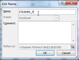
5. You should see one generic item in the list, like “Table4”.  Select this table from the list and click on the “Edit…” button.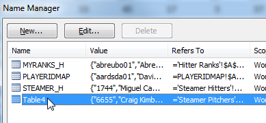Give the table a meaningful name, like “STEAMER_P” to indicate these are the Steamer Pitcher projections.  Click “OK” to close the “Edit Name” menu.  Then click “Close” to exit the “Name Manager”.
6. We now have two tables containing pitching information that we will pull from, PLAYERIDMAP (information about player name, position, team) and STEAMER_P (Steamer pitching projections).  I’m going to pull from these two tables into a new tab where I’ll calculate the pitcher rankings.
7. Right click on the “Hitter Ranks” tab and select the option to “Insert…”.  Choose the “Worksheet” option and click “OK”.  
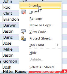
8. Right click on the new sheet tab and choose to “Rename”.  I’ll call this sheet “Pitcher Ranks”.
9. I want the first column of this new sheet to contain the Baseball Reference player ID (e.g. “strasst01” for Stephen Strasburg).  The PLAYERIDMAP sheet has a list of all fantasy-relevant players (for standard rotisserie leagues, at least).  However, this sheet contains hitters also.  Because this sheet is an Excel table, it’s easy to filter out those hitters.  Click on the drop down arrow on the “POS” column.  You’ll be presented with a list of all the positions.  Uncheck any position player and check the “RP”, “SP”, “P” values.  Click OK to apply.
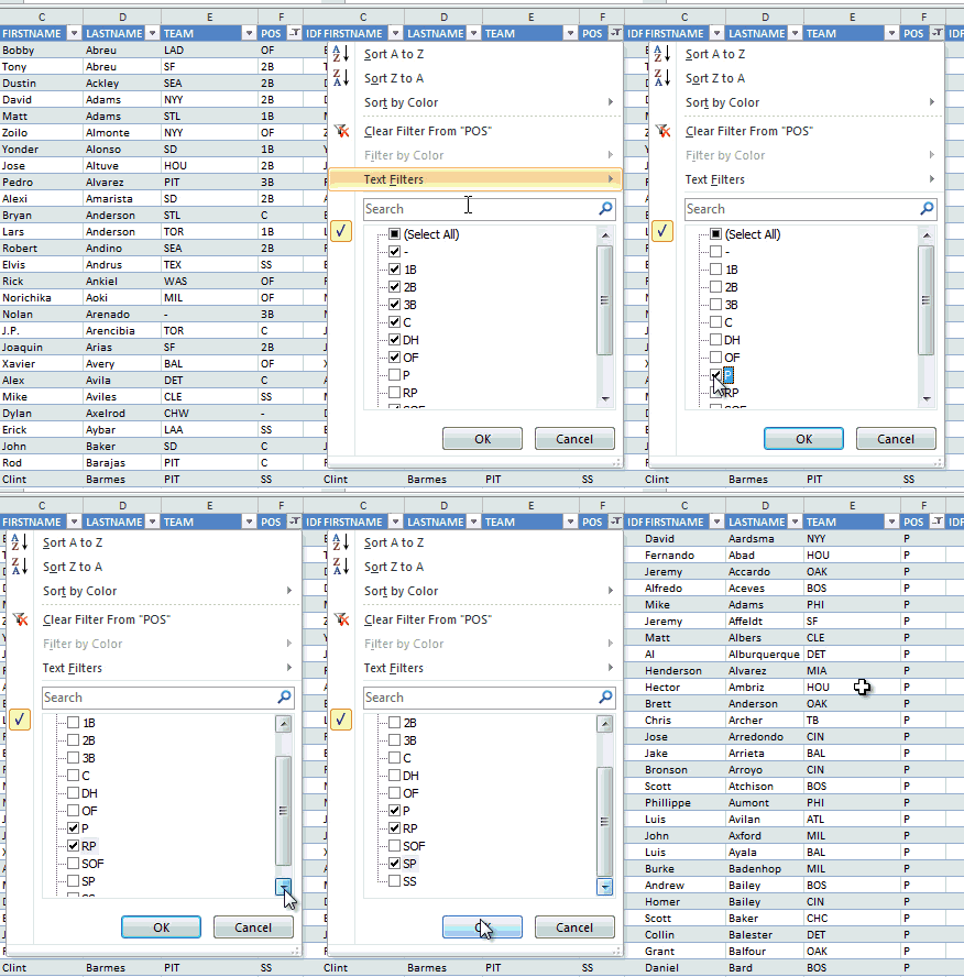
10. Starting with the first player and ending with the last, click and drag within the “IDPLAYER” column (first column) and select all players.  Only select from this first column.
    
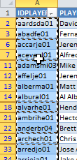
11. Copy this selected data.   Return to the “Pitcher Ranks” sheet.  Type “PLAYERID” into cell A1 (to label the column).  Then paste the data into cell A2.
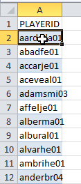
12. Because this is a new sheet, we need to convert it to an Excel table.  We will essentially repeat step 2 above, but for this different worksheet.  Click once to select any player ID.  Then locate the “Home” tab in the Excel menu system (“the ribbon”).  Click once on the “Format as Table” drop down, and then select your desired color scheme.
13. You will then be prompted to verify the range of cells in the table and that your table has a header row (which we added in step 11).  Check “My table has headers”.  Click OK.
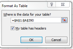
14. Repeat steps 4-6 above to give the table a more meaningful name.  In my example, Excel defaulted the table name to “Table5”.  I renamed mine to be “MYRANKS_P” (to indicate pitcher ranks).
15. Now let’s start pulling data from the other tabs.  If you need more explanation of the formulas used, refer to Part 3 of the series.  Use the VLOOKUP formula to pull  LASTNAME, FIRSTNAME, TEAM, POS, and IDFANGRAPHS from the PLAYERIDMAP table.  To get you started, an example formula to pull LASTNAME is shown here:
    

    =VLOOKUP([@PLAYERID],PLAYERIDMAP,COLUMN(PLAYERIDMAP[LASTNAME]),FALSE)
    

    

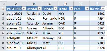
16. We’ve now pulled all the relevant information from PLAYERIDMAP and can now begin pulling in pitcher projections.  Add columns and VLOOKUP formulas to pull wins (W), games started (GS), saves (SV), innings pitched (IP), hits allowed (H), earned runs allowed (ER), home runs allowed (HR), strikeouts (SO), walks (BB), and fielding independent pitching (FIP).There will be some tweaks to the VLOOKUP formula we used earlier.  First, the Steamer projections use Fangraphs ID numbers.  So we will be using the IDFANGRAPHS column as the Lookup_value.  Second, we must specify to pull from the Steamer Pitchers projections (STEAMER_P table name).  And finally, the COLUMN formula will change to determine what statistic to pull.
    

    =VLOOKUP([@IDFANGRAPHS],STEAMER_P,COLUMN(STEAMER_P[W]),FALSE)

     

17. I don’t pull ERA or WHIP because they are rate statistics.  I prefer to recalculate them with a formula after the underlying statistics have been pulled.  That way, if I change the projections for a player, the ERA and WHIP will automatically recalculate with the updated projections.  I make an exception for FIP.  My guess is that FIP is the underlying projection that Steamer would base the ERA projection on.  I’m not doing my own projection of FIP, so I’ll leave it as is.To add ERA, type “ERA” in as a column header.  Then enter the formula to calculate ERA (ER * 9 / IP).
    To add WHIP, type “WHIP” in as a column header.  Then enter the formula to calculate WHIP ((BB + H)/IP).
    
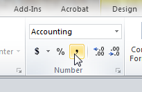
18. Most statistics don’t need formatting, but ERA and WHIP will.  Click and drag on the column headers for ERA and WHIP(“Q” and “R”, likely) to select them.  Then on the Home tab of the ribbon, click on the comma number format.
19. We’ve now successfully combined player information and projected stats into one table.

WRAP UP

Most of the hard work is done at this point.  We now have long lists of players and their projected stats.  But how do we rank them?

In the next part of the series we’ll discuss a method of evaluating a player’s projected stats and determining a ranking based upon those stats.

Please ask questions below.  Stay smart.

LINK TO DOWNLOAD FILE:  SFBB Rankings – Part 4.xlsx

IF YOU’VE MADE IT THIS FAR…

You might be interested to know that I’ve recently completed parts 7 through 10 of the “Create Your Own Rankings” series.  These additional segments include the calculation of dollar values and incorporate calculations for keeper and in-draft inflation.  All ten parts of the book are now available in Kindle format at Amazon. Please click here to read about these additions to the guide and how you can purchase all 10 parts.  My hope is that this series is the best step-by-step guide to calculating SGP-based dollar values and inflation is available anywhere.