Create Your Own Fantasy Baseball Rankings: Part 3 – VLOOKUP, Excel Tables, Named Ranges

Welcome to the third part of the “Create Your Own Fantasy Baseball Rankings” series.  If you missed an earlier part, you can find it here.  You can start at the beginning of the series or if you want to start here at Part 3, you can download the Excel file created during part 2 here.

Please note that this six part series has been adapted into a 10 part book that also shows you how to convert standings gain points into dollar values and how to calculate in-draft inflation.

A few notes about the series:

• It was originally written before the 2013 MLB season.  The screenshots and player references you see might refer to things from that time frame, but the same approach will work today.
• If you register as SFBB Insider, you can receive all six parts in a free, tidy, and easy-to-use e-book
• Familiarity with Excel is recommended, but I do my best to explain all formulas and functions used
• Some of the formulas used in the series do not work in Excel for Mac computers.  I apologize for this.  I don’t understand why Excel isn’t built to operate the same on that platform.

In this third part of the series we will use Excel formulas and functions to start pulling player information (name, position, team) and projection information in order to eventually calculate our own rankings.  Strap in…  This is a long one.

Excel Functions and Formulas In This Post

Below are the Excel functions and formulas used in this part of the series.  If you’re already familiar with what these are, you can skip ahead.

VLOOKUP

One of the most powerful Excel formulas, in my opinion.  And it’s easier to use than you might think.  This formula searches the first column of a table for a desired value (a player ID) and then returns a value that is in the same row but in a separate column.  For example, we might tell Excel to go into a table of projection data, locate a specific player ID, and give us back the number in the eighth column (which holds the number of HRs).

This formula requires four inputs:

VLOOKUP(lookup_value, table_array, col_index_num, range_lookup)

1. lookup_value – This is the value to search for.  In the rankings spreadsheet, we’re mostly going to use player IDs for this.  “Hey Excel, go look for this player ID”.
2. table_array – This has to be two or more columns of data.  Excel will look for the look_up value in the first column in the set of data.  You do not necessarily need to include the first column on a spreadsheet tab.  But Excel is going to look through the first column you provide.  “Hey Excel, here are ten columns of data for you, look through everything in the first column for the lookup_value.”
3. col_index_num – This is the column number from the table_array that contains your desired information.  This has to be a number and it has to be within the table_array you provided.  For example, if your table_array only has five columns, but you put a 6 for col_index_num, you’ll have a problem.  “Hey Excel, the eighth column has projected home runs.    Tell me how many home runs are projected for this player ID.”
4. range_lookup – This input can be either “TRUE” or “FALSE”.  If you use “TRUE”, Excel will look for an approximate match of the lookup_value (PLAYERID).  If you enter “FALSE”, Excel will only look for an exact match.  This is an optional input, but I feel very strongly that it must be used and that “FALSE” is the option selected.  You may otherwise get the wrong projections showing up for players.

TABLES (NAMED RANGES)

Excel has functionality that allows you to convert a block of data (player projections) into a table.  There are quite a few benefits to using tables:

1. Tables can have names.  This is great for the table_array input in the VLOOKUP formula.  We can give the projection sheet the name “STEAMER_H” (for Steamer Hitters projections) and use that instead of traditional way of selecting data in Excel (something like ‘Steamer Hitters’!A1:W500).
2. Columns have names.  I have a hard time remembering what column projected HRs are in.  But I don’t need to if I know that the column name is “HR”.  If you don’t use a table, you’re stuck trying to remember things like, “were HRs in column G, H, or I?”.  When referring to a column, use the following convention – TABLENAME[COLUMNNAME].  The column name is surrounded in brackets.
3. Easily adding calculations.  In a table, all formulas within a column are identical.  This is great for consistency.  And because of this, when you change the formula in one cell of a column, the rest of the column automatically updates too.  No more editing a formula in one cell and having to copy it to hundreds of other cells.
4. Easy sorting and filtering.  As easy as clicking a drop down arrow.

COlumn

This function returns the column number of a cell or range of data.  The function only requires one input; the cell or range to be evaluated.  For example:

COLUMN(TableName[ColumnName]) selects an entire column from a table and will return the column number.

 STEP-BY-STEP INSTRUCTIONS

1. In Part 1 of this series I showed you how easy it is to find some high quality projection data for free.  For the sake of simplicity, I’m going to pick one source to move forward with.  This smart article at Razzball reviews the accuracy of 2012 projections and puts the Steamer projections in a positive light.  So I’m going to move forward and base my rankings off of Steamer.  You can choose whatever source you prefer.
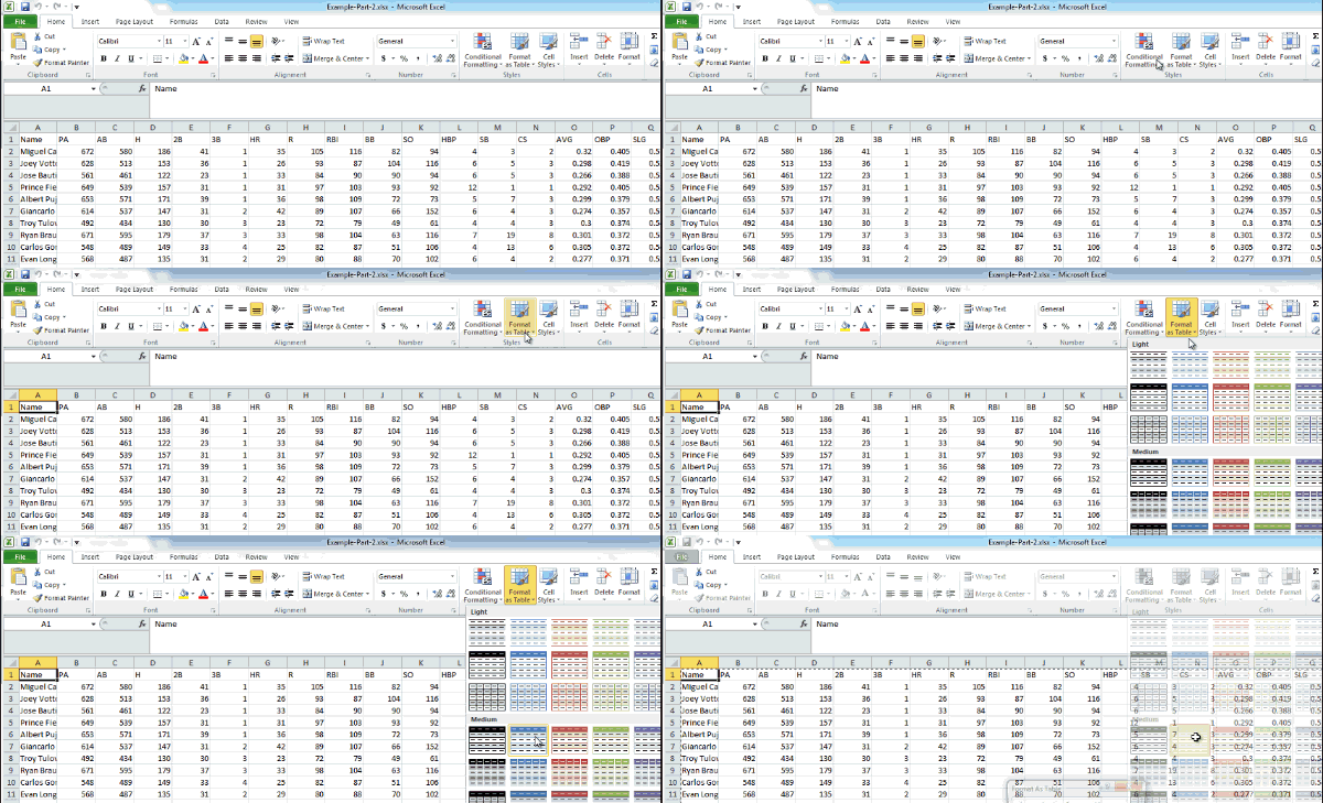
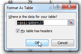
2. To make the projections easier to work with, convert the “Steamer Hitters” tab to a “table” in Excel.  Click anywhere within the data on your hitter projection worksheet.  Then locate the “Home” tab in the Excel menu system (“the ribbon”).  Click once on the “Format as Table” drop down, and then select your desired color scheme.You will then be prompted to verify the range of cells in the table and that your table has a header row (e.g. Name, AB, H, HR, etc.).  Check “My table has headers”.  Click OK.
   
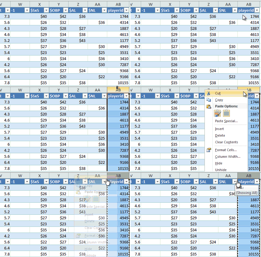
   After accepting this, your bland looking data will transform into a nicely formatted table.
3. We’ll later be pulling information from this table into other worksheets.  To make the pulling of data easier we need to move the fangraphs player ID to be the first column (you can use VLOOKUP if the player ID is in the first column, otherwise you’re stuck using more difficult and/or multiple formulas).  Right-click on the top of the fangraphs player ID column (I right clicked on the “AB” column header, not for At Bats, as in the column next to column “AA”) and Cut it.
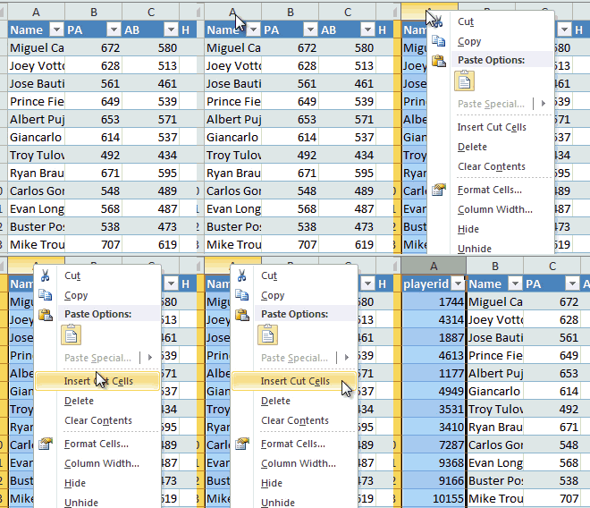
4. Now right-click on the top of the player name column (column header “A”) and select “Insert Cut Cells”.
5. Before we finalize this table, we must give it a name.  Go to the “Formulas” tab on the Excel ribbon and click on the “Name Manager” button.
6. Excel will give very generic names to a table, like “Table2”.  It’s more helpful to give meaningful names to your tables.  As you get more tables in a spreadsheet, it can become very difficult to remember the difference between “Table2” and “Table3”.  Note how there is already a table named “PLAYERIDMAP”.  I previously set up this table before you inserted it into your Excel file in Part 2 of this series.  Select your table from the list and click on the “Edit…” button.
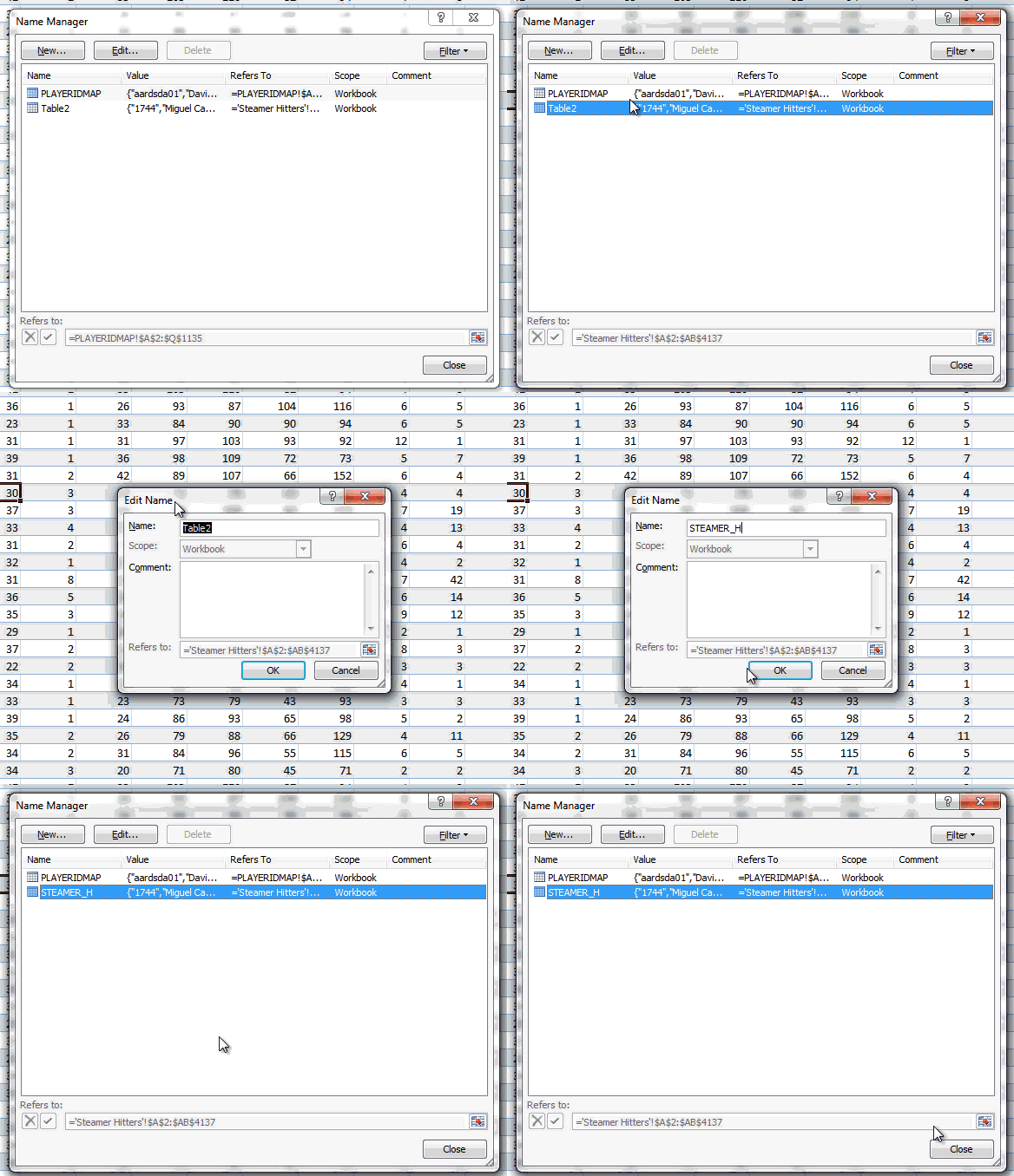
7. Give the table a meaningful name.  I chose “STEAMER_H” to indicate these are the Steamer Hitter projections.  Click “OK” to close the “Edit Name” menu.  Then click “Close” to exit the “Name Manager”.
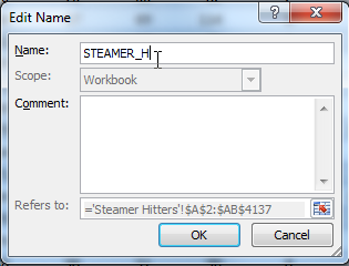
8. We now have two tables ready to pull information from, PLAYERIDMAP and STEAMER_H.  I’m going to pull from these two tables into a new tab where I’ll calculate the hitter rankings.
9. Right click on the “PLAYERIDMAP” tab and select the option to “Insert…”.  Choose the “Worksheet” option and click “OK”.  
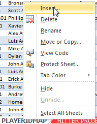
10. Right click on the new sheet tab and choose to “Rename”.  I’ll call this sheet “Hitter Ranks”.
11. I want the first column of this new sheet to contain the Baseball Reference player ID (e.g. cabremi01).  I believe the PLAYERIDMAP sheet has a list of all fantasy-relevant players (for standard rotisserie leagues, at least).  However, this sheet contains pitchers also.  Because this sheet is an Excel table, it’s easy to filter out those pitchers.  Click on the drop down arrow on the “POS” column.  You’ll be presented with a list of all the positions.  Uncheck any “RP”, “SP”, “P” values (Note:  at some point during 2014 I stopped classifying pitchers in these categories and now just track all as “P”).  Click OK to apply.
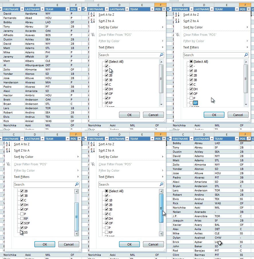
12. The Player ID Map will now list only hitters.  Starting at the first player and ending with the last, click and drag within the “IDPLAYER” column (first column) and select all player (or select the first player and then use the keyboard shortcut SHIFT + CTRL + Down Arrow).  Only select from this first column.
    
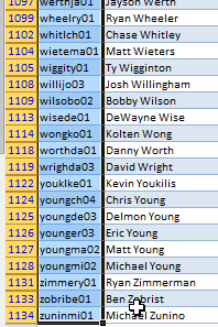
13. Copy this selected data.   Return to the “Hitter Ranks” sheet.  Type “PLAYERID” into cell A1 (to label the column).  Then paste the data into cell A2.
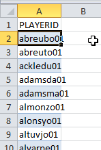
14. Now that we’re starting this new sheet, we should convert it to an Excel table.  We will essentially repeat step 2 above, but for this different worksheet.  Click once to select any player ID.  Then locate the “Home” tab in the Excel menu system (“the ribbon”).  Click once on the “Format as Table” drop down, and then select your desired color scheme.
15. You will then be prompted to verify the range of cells in the table and that your table has a header row (which we added in step 13).  Check “My table has headers”.  Click OK.
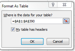
16. Repeat steps 5-7 in order to give the table a more meaningful name.  In my example, Excel defaulted the table name to “Table3”.  I renamed mine to be “MYRANKS_H” (to indicate hitter ranks, because we’ll also be ranking pitchers).
17. Now for the fun part…  pulling data from the other tabs.  I’ll first add “Player Last Name” to the table.  To expand your table, simply type into column B and hit Enter (I typed into cell B1).  Excel should automatically pull this new column into your table.  I’m going to name my column “LNAME”.
18. Our goal in this column is to instruct Excel to take the PLAYERID from column A, go into the first column of PLAYERIDMAP, find the matching PLAYERID, and then pull the corresponding LASTNAME.  You can see in the image of the PLAYERIDMAP below that LASTNAME is in the fourth column (column D).To start building the formula, click in cell B2 of your Hitter Ranks tab.  Then click the “fx” button of the formula bar to launch Excel’s formula wizard.  We’ll use the wizard the first time through to better explain this function in Excel.
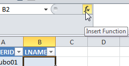
19. Type “vlookup” into the search bar and click “Go”.  When the function appears, make sure it is selected and hit “OK”.You should then see the different arguments, or components, needed for the formula to work.  
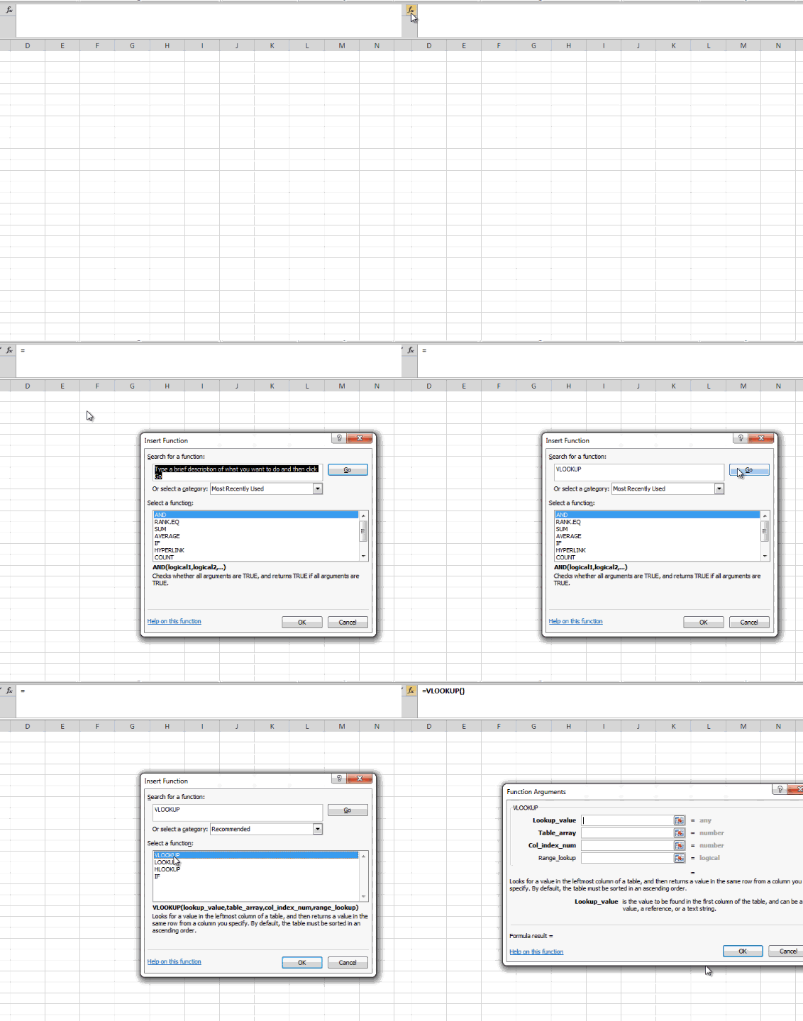
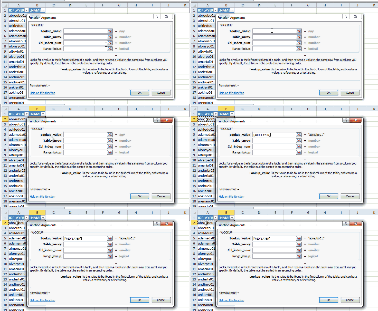
20. The “Lookup_value” is the value on the “Hitter Ranks” sheet that we want to locate in “PLAYERIDMAP”.  Click once in the “Lookup_value” field.  Then click on the value in cell A2 (“abreubo01”).  Excel will convert this to [@PLAYERID].  This naming convention can be used when you have converted your date into an Excel table.  If you can’t remember the naming convention, you can always use this formula wizard to build formulas.
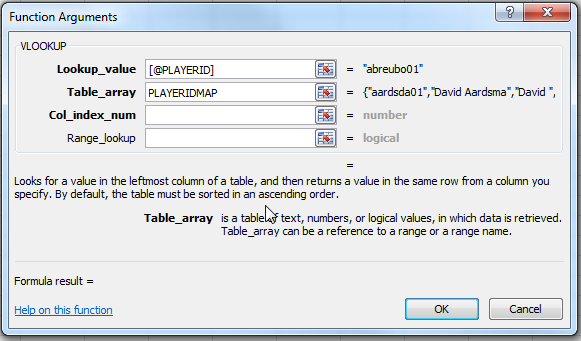
21. The “Table_array” field is the table in which to go look for the matching PLAYERID.  Click once in the “Table_array” field.  Simply type “PLAYERIDMAP” (no quotes).  Again, this is another benefit of using Excel tables.  It’s much easier to type in the table name than it is to flip tabs in Excel and select a giant range of data.
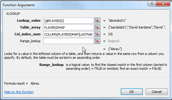
22. The “Col_index_num” field wants to know the number of the column in the PLAYERID map table to retrieve data from.  Again, our goal is to retrieve LASTNAME from the PLAYERIDMAP table, which is column 4.   You could manually flip back and forth between tabs to determine the column number.  You could then enter a 4 in for “Col_index_num”.  This takes time and can be difficult if you start getting into column X (do you know what number letter of the alphabet that is?).Alternatively, I prefer to use the COLUMN function.  When the COLUMN formula  is entered into the Col_index_num field, it will return the column number.  The formula below will determine that LASTNAME is the fourth column in the PLAYERIDMAP table.
    

    COLUMN(PLAYERIDMAP[LASTNAME])

    Enter this equation into the Col_index_num field.

23. Finally, we have the Range_lookup argument.  I always enter “FALSE” for this in order to ensure Excel only locates exact matches for a PLAYERID.  I don’t want Excel to return an approximate match if the exact PLAYERID cannot be found.
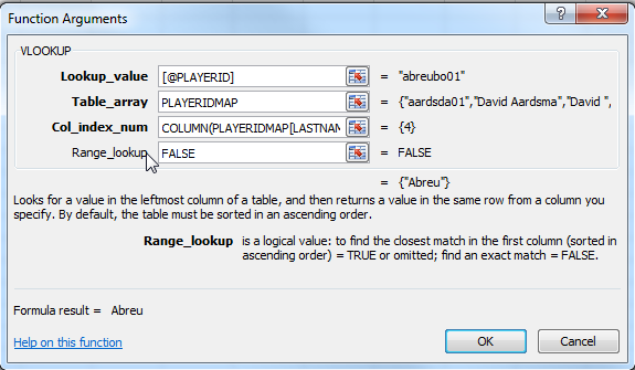
24. Before hitting “OK” to accept the formula, you can preview the output.  In this case we are dealing with “abreubo01”, or Bobby Abreu, and can see the formula appears to be working.  Click OK to accept the formula.
    
25. Once the formula is entered, it should automatically copy to the remaining rows of the table.
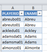
26.  We will use the VLOOKUP formula to pull additional data, and the majority of the formula will remain the same.  To add a FNAME column, type the column name into cell C1.  Copy the formula from cell B2 (actually copy it from the formula editor bar, click ESC to exit the formula editor).    Paste the formula into cell C2.  Then simply change the column name (remember column names are surrounded in [brackets].  So change [LASTNAME] to [FIRSTNAME].
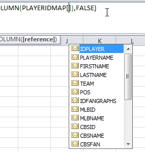
27. Repeat step 26 to pull TEAM, POS, and IDFANGRAPHS from the PLAYERIDMAP tab.  If you can’t remember the exact name of a column, once you have entered a table name, like PLAYERIDMAP, and the opening “[” bracket, a helpful type ahead box will display all the column names in the PLAYERIDMAP table.
28. We’ve now pulled all the relevant information from PLAYERIDMAP and can now begin pulling in hitter projections.  Add columns and VLOOKUP formulas to pull plate appearances (PA), at bats (AB), hits (H), home runs (HR), runs (R), runs batted in (RBI), walks (BB), strikeouts (SO), and stolen bases (SB).There will be some tweaks to the VLOOKUP formula we used earlier.  First, the Steamer projections use Fangraphs ID numbers.  So we will be using the IDFANGRAPHS column as the Lookup_value.  Second, we must specify to pull from the Steamer Hitters projections (STEAMER_H table name).  And finally, the COLUMN formula will change to determine what statistic to pull.
    

    =VLOOKUP([@IDFANGRAPHS],STEAMER_H,COLUMN(STEAMER_H[PA]),FALSE)

     

29. I don’t pull average or any other rate statistics (OBP, SLG, etc.).  I prefer to recalculate them with a formula after the underlying statistics have been pulled.  To do this, type “AVG” in as a column header.  Then enter the formula to calculate batting average (H divided by AB).  
30. Most statistics don’t need formatting, but AVG will.  Click on the “P” to select the entire AVG column.  
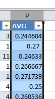
    Then on the Home tab of the ribbon, click on the comma number format.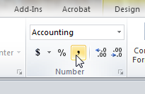Finally, click on the symbol to increase the decimal places from 2 to 3.
    
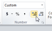
31. We’ve now successfully combined player information and projected stats into one table.  
    

 WRAP UP

This was a long one…  Stick with it.  In the next part of the series we’ll reperform many of these steps in order to create a pitchers ranks table.  It will be a more abbreviated post that will only touch on the key differences needed for pitchers.

Please ask questions below.  And as always, make smart choices.

Link To Download File:  SFBB Rankings – Part 3.XLSX

IF YOU’VE MADE IT THIS FAR…

You might be interested to know that I’ve recently completed parts 7 through 10 of the “Create Your Own Rankings” series.  These additional segments include the calculation of dollar values and incorporate calculations for keeper and in-draft inflation.  All ten parts of the book are now available in Kindle format at Amazon. Please click here to read about these additions to the guide and how you can purchase all 10 parts.  My hope is that this series is the best step-by-step guide to calculating SGP-based dollar values and inflation is available anywhere.